Services on Demand
Article
Estudios Económicos
On-line version ISSN 2525-1295
Estud. Econ. vol.36 no.72 Bahía Blanca Jan. 2019
Commodities prices and critical parameters for macroeconomic performance: a CGE analysis for Argentina, Brazil and Chile°
Precios de commodities y parámetros críticos para el desempeño macroeconómico: un análisis de equilibrio general computado para Argentina, Brasil y Chile
Omar O. Chisari* - Leonardo J. Mastronardi** - Carlos A. Romero***
* Instituto Interdisciplinario de Economía Política de Buenos Aires (IIEP-BAIRES), Facultad de Ciencias Económicas, Universidad de Buenos Aires and CONICET.
** Facultad de Ciencias Económicas, Universidad Nacional de La Plata e Instituto de Economía, Universidad Argentina de la Empresa.
*** Instituto Interdisciplinario de Economía Política de Buenos Aires (IIEP-BAIRES), Facultad de Ciencias Económicas, Universidad de Buenos Aires. Correo electrónico: carlos.adrian.romero@gmail.com
enviado: 14 febrero 2018
aceptado: 29 octubre 2018
Abstract
We study the potential performance of Argentina, Chile and Brazil, following a reduction of prices of exports and imports of commodities. To that aim, we construct three CGE models based on the same analytical framework. The impact of low commodities prices depends on the share of exports in GDP, the share of exports of commodities in total exports, the import-intensity of manufactures and the share of labor in GDP. We find that Argentina is vulnerable to the reduction of prices of commodities because it is highly dependent on exports of agricultural commodities and/or their derivatives. Chile is vulnerable to price reductions of copper even though its economy is protected by a sound macroeconomic policy and because its economy is less labor-intensive than the others. Brazil would be the less affected by a generalized fall of commodities prices since its economy is more diversified.
JEL Code: D58.
Keywords: Computable General Equilibrium; Prices of Commodities.
Resumen
Estudiamos el desempeño potencial de la Argentina, Chile y Brasil como resultado de una reducción de precios de la exportación e importación de bienes en mercados competitivos internacionales. Para ese fin, construimos tres modelos de Equilibrio General Computado basados sobre una estructura analítica similar. El impacto de bajos precios de dichos bienes depende de la participación de las exportaciones en el PBI, de su participación en el total de exportaciones, de la intensidad en importaciones de las industrias manufactureras y de la participación del trabajo en el PBI. Encontramos que la Argentina es vulnerable a la reducción del precio de los commodities porque es altamente dependiente de las exportaciones agrícolas y de sus derivados. Chile es vulnerable a reducciones del precio del cobre aun cuando su economía está protegida por una correcta política macroeconómica y porque su economía es menos trabajo-intensiva que la de los otros países. Y Brasil sería menos afectado por una caída generalizada de precios pues su economía está más diversificada.
Código JEL: D58.
Palabras clave: equilibrio general computado, precio de commodities.
INTRODUCTION
Prices of commodities have an important influence on the growth of less developed economies and impact on the welfare of the poor. High prices of commodities, in particular those of food and agricultural products, reduce the welfare of import countries.
However, little effort has been devoted to analyze the vulnerability of export countries. This is relevant because low prices of commodities can reduce the welfare of the poor too, in the context of macroeconomic adjustment, and could jeopardize the efforts made by those economies to reach higher rates of growth.
In this paper, we discuss the cases of three Latin American economies: Argentina, Brazil and Chile. All of them have a significant dependence of their macroeconomic performance with respect to the commodities prices level and volatility. The countries selected for the study represent three different economic structures, though they are among the most advanced of South America. Argentina still struggles to diversify exports that are concentrated basically in agricultural products and their derivatives. Brazil has reached a higher degree of diversification, but it is very dependent on imports of inputs for manufactures. And Chile is the most modern economy in services, but it is still dependent on exports of mineral products. Particularly, soybean has a very important share in total exports of Argentina, and copper has a similar role for Chile, while Brazil is less specialized, but still very dependent on export prices and highly sensitive to import prices of commodities for the manufacturing sector.
Fiscal result is also very much linked to commodity prices in the three economies. In Argentina, there exist export taxes that represent 8% of total revenue and commodities sectors pay approximately 40% of the indirect taxes. In the case of Chile, the public sector owns 31% of total capital in the mining sector, and commodities sectors pay approximately 42% of the indirect taxes. In Brazil, 23% of the total indirect taxes revenue is obtained from the production of commodities.
We present the results of the computable general equilibrium model constructed for those economies and the results of simulations that assume that the bonanza period for commodities ends with a reduction of ten percent in their prices (in real terms)1. It will be seen that the impact on the economies are significant, and it depends on four main indicators: the coefficient of openness, the share of commodities in total exports and imports, and the share of labor in GDP.
Thus, we explore the answers and the elements that explain them with respect to the following questions: How will the economies react to a reduction of international prices of commodities? How will the results change to a similar reduction of prices of imports? Does the response depend on the capital/labor ratio? Will there be relevant differences when wages are adjusted in real or nominal terms? Will the mobility of capital be relevant for the results?
The results of the simulations indicate that the economy of Argentina is vulnerable to a reduction of prices of commodities because it is dependent on exports of agricultural commodities or their derivatives (like soybean and soybean oil). In addition, these results show that downward inflexibility of nominal wages can amplify the shock, because the economy is labor-intensive. Chile is vulnerable to price reductions because it is highly dependent on prices of copper and because it does take advantage of import prices reductions to a limited extent. However, Chile has developed contingent funds and the economy is less labor-intensive. Brazil would be the less affected by falls of commodities prices because its economy is more diversified, where the manufacturing sector could be benefitted by reductions of prices of imported inputs.
The paper is organized as follows. Section 2 provides a summary of the data used and the procedure of construction of the Social Accounting Matrices as well as of the main indicators; the SAMs are included in the appendix. Section 3 presents the basic model, and Section 4 shows the results obtained in the simulations. Section 5 discusses the main lessons and conclusions.
I. DATA AND SOCIAL ACCOUNTING MATRICES
The model has a Walrasian structure, adapted to take into account macroeconomic effects. It has been used for studying tax incidence, macroeconomic shocks and impact of regulation of utilities (Chisari, Romero and Estache, 1999; Chisari et al., 2012 and 2013). The modeling begins with the construction of the Social Accounting Matrix, the analytical structure and its transcription in terms of the MPSGE (Mathematical Programming System for General Equilibrium). MPSGE was developed by T. Rutherford (U. of Colorado) in 1987. He showed that a Computable General Equilibrium (CGE) model can be represented as a Mixed Complementary Problem. At present, MPSGE is used in interface with GAMS (General Algebraic Modelling System). The CGE models have all the basic properties of the Walrasian perspective, and they are numerically solved using the GAMS/MPSGE program.2
As said above, the first step is to develop a Social Accounting Matrix (SAM) of the economy to consistently combine and summarize the information on major macroeconomic transactions. The matrix covers four types of markets-the domestic production and investment market (for final and intermediate use), the investment goods market, the labor market and the bonds (or credit) market. Every productive sector is represented by a firm that manufactures only one product with a constant-return to scale production function, both for goods and services. The firms hire labor and capital which are endowments of households and of the foreign sector. The public sector demands goods and labor and offers bonds for amounts equivalent to the level of expenditures not covered by tax revenue.
The demand sides were modeled through two representative households, a government, and an external sector. Households buy or sell bonds, invest, and consume in constant proportions (Cobb-Douglas) given the remuneration for the factors they own (and the government transfers they receive). The choice of the optimal proportion of the consumption good is obtained from a nested production function in the utility function through a cost minimization process. For private agents and the public sector, welfare changes are calculated using the Equivalent Variation. Our interpretation is that this would represent a monetary proxy of changes in the society's welfare resulting from modifications in the availability of goods and services provided by the public sector (e.g., education, health and defense). The simple change of revenue would not take into account variations in the prices of goods, services and factors, and the Equivalent Variation instead helps to provide an estimate of those changes.
Government is represented as an agent that participates in markets for investments, consumes, and makes transfers to households and has a Cobb-Douglas utility function; its main source of income is tax collection (though it also makes financial transactions through the bonds account). The rest of the goods are taken as complementary, and the elasticity of substitution between them is zero. Therefore, we have a Cobb-Douglas utility function attributed to the government; this choice was motivated by the property of the Cobb-Douglas function of leaving constant the share of every kind of expenses in the total, which seemed to be a neutral way of modeling the behavior of the government. Thus it is assumed that each dollar of revenue is spent on different factors and goods in the same proportion as in the benchmark.
The economies were assumed to be small with respect to international markets. The rest of the world buys domestic exports and sells imports, in addition to making transactions of bonds and collecting dividends from investments. The social accounting matrixes show that Argentina, Brazil and Chile had a trade surplus for the benchmark year. Then it was assumed for the simulations that the trade surplus is positive and a constant proportion of the GDP.
With respect to the supply side, the production function in each sector is a Leontief function between value added and intermediate inputs: one output unit requires x percent of an aggregate of productive factors (labor, non-mobile capital, mobile capital, and land) and (1-x) percent of intermediate inputs. The intermediate inputs function is a Leontief function of all goods, which are a strict complement in production. By contrast, value added is a Cobb-Douglas function of productive factors. Private, public and foreign savings are totaled to finance investments.
The construction of the SAM is very demanding in terms of data. The main sources of information are the national accounts and the input-output matrix, complemented with information from the internal revenue services and surveys of consumption expenditure and income distribution when available. Those sources are quoted in the references.
To understand the information included in the SAM, notice that columns present expenses of agents or sectors, while rows show demand of a good or service distributed for every agent in every market. The total of a row must then be equal to the total of a column (the total of expenditure in a good or service must be equal to the total of revenue for that good or service).
After the construction, it is necessary to calibrate the matrix and the model. Since the sources of information might differ or the data of the input-output table could be not updated, there is a first round of calibration of the inter-sector transaction matrix using RAS. A second round of calibration, for the model itself, is performed previously to simulations to determine the implicit scale factors, shares or elasticities of substitution to replicate the benchmark year. For this second procedure, MPSGE is used. Finally, after the simulations, the information is transformed and presented with the macroeconomic aggregates since the solution of the model is basically an equilibrium vector or relative prices, i.e. relative prices that obtain simultaneous clearing of all markets.
Since positive unemployment is observed in the benchmark year the labor market requires a special treatment. It is necessary to define a rule of adjustment of wages, because the market forces are not operating. Thus we contemplate two cases. The first one considers that wages are downward inflexible in real terms, which means that they are both downward and upward flexible in nominal terms. The second case assumes that wages are downward inflexible in nominal terms. The implications for the simulations are dramatic; for example, when commodities prices are reduced and wages are nominally fixed, the reduction of employment is much bigger than in the case when wages are adjusted nominally though fixed in real terms, and the reduction of GDP is also very significant. Table 1 shows the composition of value added for the economies of the countries in this paper3.
Table 1. Composition of value added for the economies of the countries in this paper
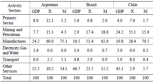
Sectoral shares of GDP (% of total).
Source: own elaboration using data included in the SAM.
Note: "X" corresponds to Exports and "M" corresponds to imports.
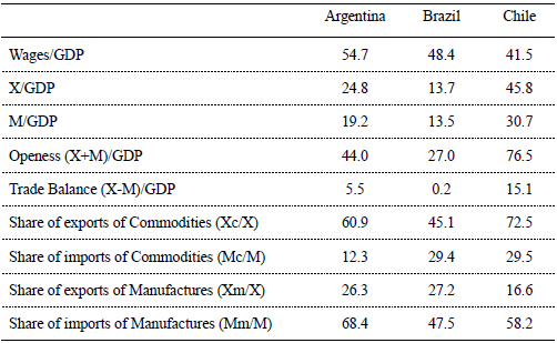
Some structural characteristics have a role for the results to be obtained, as indicated by Céspedes and Velasco (2012). There are some key indicators that will help to understand the results of simulations. Table 2 shows four indicators: the share of exports and imports in GDP, the share of commodities in total exports and imports, and finally the share of labor in GDP. The first one is relevant because it gives the openness of the economy, and the sensitivity to external shocks should be higher the greater the coefficient of openness.
Table 2. Main indicators of the countries (%)
Source: own elaboration using data included in the SAM
The share of commodities in total exports is also relevant, since if exports did not include a big proportion of commodities, the economy would be immune to reductions of commodities price. That is not the case of Chile, since that country has a high coefficient of openness and a high share of commodities (mainly copper) in total exports. This explains the special care of authorities for the construction of compensatory mechanisms (accumulation of ear-marked funds to stabilize shock from the rest of the world).
The third indicator will explain why some of the countries could benefit from reductions in the prices of commodities; that will happen when production is imports-intensive. That is what is observed for Brazil. Finally, the share of labor will help to understand some big differences in the results among the countries, when the simulations assume nominal or real wages. The adjustment of wages will become also relevant in the comparison between countries, when goods that enter in the consumption basket or the price index are also export-goods, as it is the case of Argentina.
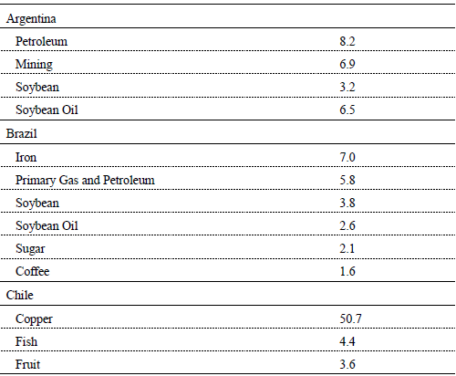
Table 3 shows the most important export commodities for the three countries. It also shows the share of commodities in exports for each one of the categories. For example, in the case of Chile, exports of mining represent approximately 55% of total exports (see Table 1), and of that, 92% correspond to copper (see De Gregorio and Labbé (2011)). In the case of Brazil, even though soybean has an important role in total exports, agricultural exports are below 7% of the total. In the case of Argentina, exports of soybean represent 26% of the 12% corresponding to agricultural exports, but that share should be increased when soybean oil were included (11% of total manufactures exports).
Table 3. Main export commodities (% of total country exports)
Source: own elaboration using data included in the SAM.
II. THE MODEL IN A NUTSHELL
In this section we present a brief discussion of the basic elements of the model in a simplified version. Though we have in general two agents in our CGE models, let us assume that there is only one representative household that maximizes utility.
Equation (1) gives the equalization of the subjective rate of substitution with relative prices, corrected by ad valorem taxes, in this case only charged on good 1 (the general model includes several taxes, as well as agents and goods).
 | (1) |
Equation (2) gives the budget constraint. It is assumed that there is only one kind of labor, L0 (W is the wage rate), but two kinds of capital-fixed and mobile-between industries. There is one unit of specific capital in each industry, and its prices are indicated with πi (alternatively, this can be interpreted as total profits of the sector with constant returns to scale). The endowment of internationally mobile capital, owned by the domestic household, is given by K0 and its remuneration is R*. At the benchmark, the proportion of fixed capital owned by the domestic household with respect to mobile capital is therefore 2/K0 (in fact, this parameter can be unobservable and uncertain).
 | (2) |
Equations (3) to (6) give the definition of profits for sector 1, the production function, and the optimal benefits first order conditions, respectively. The price received by producers is net of expenses in intermediate inputs, both domestic and imported (given by a, and α). Imported goods are used as the numeraire. Equations (7) to (10) are the analogous equations for sector 2.
 | (3) |
 | (4) |
 | (5) |
 | (6) |
 | (7) |
 | (8) |
 | (9) |
 | (10) |
Equation (11) represents the budget condition for the public sector; in this simplified case, it is assumed that all revenue is used to hire labor (the general model includes purchase of goods, transfers to households, investments, and net changes in the financial result).
 | (11) |
Equations (12) to (15) are the equilibrium market conditions. The first one includes exports, x; the third equation determines unemployment, un, and the last equation gives the equalization of demand and supply of mobile capital.
 | (12) |
 | (13) |
 | (14) |
 | (15) |
Equation (16) fixes the price of good 1 at the level given by the rest of the world because it is a tradable good (this is the case of a small economy).
 | (16) |
Equation (17) represents nominal wages determination as a weighted average of prices of tradable goods, non-tradable goods (and imports in the general model).
 | (17) |
This is taken as an equation in the benchmark. In equation (18) we define imports, limited to those for industrial uses, which in this simplified version does not include imports of final goods (the CGE model includes imports of final and intermediate goods).
 | (18) |
The 18 unknown variables are: P1, C1, P2, C2, W, π1, π2, L1, L2, un, K1, K2, Q1, Q2, Lg, m, x and Km. This simplified presentation abstracts from the mechanism of adjustment of the trade balance. The general model assumes that the trade surplus is used by countries to purchase a bond issued by the rest of the world. Since those bonds enter in the utility function of the government and of the domestic agents, and those utility functions are assumed from the Cobb-Douglas form, the procedure is equivalent to assuming that the trade surplus is approximately (i.e. except for changes in income distribution) a fixed proportion of domestic GDP. Thus, in this case, a positive trade surplus cannot be reversed and becomes negative. A more detailed presentation of the model can be found in Chisari, Estache and Romero (1999) and in Chisari et al. (2013).
III. SIMULATIONS
Results are summarized using a set of indicators for the economies. We include the change of GDP and the share of exports (X) and imports (M) in GDP, the equivalent variations for the poor, the rich and the public sector. The last one is less standard, but as it has already been argued, we assume a Cobb-Douglas utility function for the government because that function implies constancy of the share of different types of expenses. And we also include the average rate of profit in primary, secondary and tertiary sectors, to appraise how the industrial structure responds or will respond to the new relative prices. CPI stands for consumer price index (benchmark = 1) and RER, for real exchange rate (as of the ratio between prices of tradables and non-tradables). Notice that the CPI falls because it is assumed that there is full downward flexibility of nominal prices, and since commodities prices are lower, the law-of-one-price implies that those prices will fall also in the domestic markets.
From the perspective of this simple version of the model, we shall consider the following comparative statics exercises:
a. Reductions of 10% of export prices4, P*, under minimum real wages (equivalent to γ3 = 0 in eq. 17) and minimum nominal wages (γ1 = γ2 = 0 in eq. 17). In the framework of our model, the main relative prices of tradables to non-tradables are given by the ratio of P* to wages. Thus, flexible nominal wages are equivalent to the possibility of devaluation.
b. Reductions of 10% of P* and of import prices, Pm, under minimum real wages (equivalent to γ3 = 0 in eq. 17) and minimum nominal wages (γ1 = γ2 = 0 in eq. 17).
Of course the potential changes in prices of commodities could be different, but it can be argued that, in that case, changes in main economic indicators will be proportional to our estimates considering the benchmark of 10%.
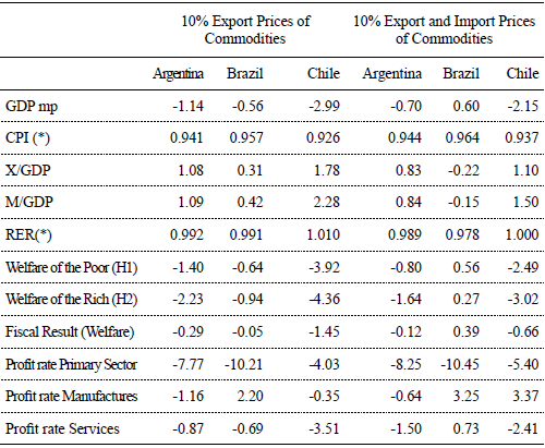
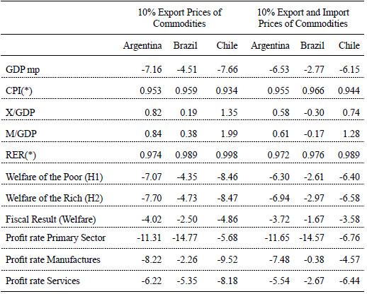
The main results are presented in tables 4 and 6. In general, the three economies suffer following the reduction of export prices, and the fall of all indicators is higher when nominal wages are considered. However, it can be seen that Chile is hit more strongly when nominal wages are flexible since its GDP falls almost 4%; this is due to its high ratio of exports to GDP. This is coincident with econometric evidence -see for example Lanteri (2009) who studied the case of Argentina.
Table 4. Results under real wages inflexibility (% of change)
(*) Level with respect to benchmark = 1. Source: own elaboration.
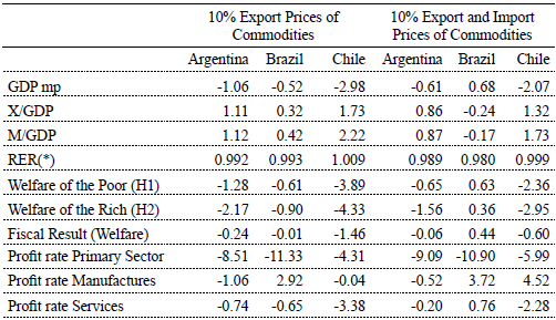
Table 5. Results under nominal wages inflexibility (% of change)
(*) Level with respect to benchmark = 1. Source: own elaboration.
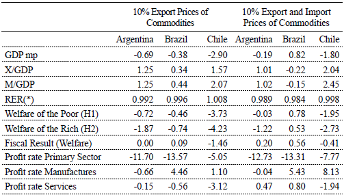
Table 6. Results under real wages inflexibility and capital mobility of 25% (% of change)
(*) Level with respect to benchmark = 1. Source: own elaboration.
Even though prices of exports are falling, it is observed that exports grow as a percentage of GDP for the three economies. The composition of export also changes depending on relative prices. This means that following the fall of prices, all the economies compensate with an increase in quantities to meet the current account equilibrium.
Inflexibility of nominal wages is key to the macroeconomic adjustment. All the indicators worsen if wages do not fall in terms of international prices (which is equivalent to say that a devaluation is not possible). The prices of tradables to non-tradables worsen as a result of the nominal inflexibility of wages. Moreover, downward inflexibility of nominal wages does not help the poor. The reason is that the level of employment falls further in all the three economies.
A simultaneous reduction of prices of imported commodites compensates the reduction of export prices, and the performance of all the three economies is improved. But this compensation is specially effective for Brazil and to a lesser extent for Argentina. This good outcome is due to the intensity of use of imported inputs by manufactures since, as can be seen in Table 1, following a reduction of all prices, the economy of Brazil has an increase of GDP. But this result is also a warning, for it indicates that an increase of prices of commodities would not necessarily be beneficial for Brazil (when the stock of capital is given, since Brazil performance in the commodities export markets in the 2000s was followed by an increase in arable land).
However, even though the economy of Chile is less resilient to import prices, manufactures of that country experience an increase of profits when import goods are reduced. The same happens for Brazil, but not in Argentina. This might be the result of a more deep relation between industries in the last case, which implies a higher correlation of profits.
In all three cases, the primary sectors see a stronger fall of their rates of profit since those sectors concentrate exports of commodities and do not benefit directly from the fall of prices of imports.
The impact on fiscal result is different between countries. Argentina and Chile experience the strongest negative result, because their fiscal revenue depends on export taxes on agriculture and profit taxes, on copper. Brazil is relatively immunized because of the diversification of its economy.
The impact on households is negative in all simulations (exception for Brazil 10% Export and Import Prices of Commodities in real wages model when the effect on GDP are compensated). The richest household is capital intensive in terms of endowments. This implies that a negative shock in profit rates reduces their welfare more strongly than the welfare of the poor. In the comparison across the countries, we observe that households from Argentina and Chile are more affected by the international shock than Brazilian households (as a consequence of a more diversified economy when international prices affect less real GDP)
1. International Prices and capital mobility
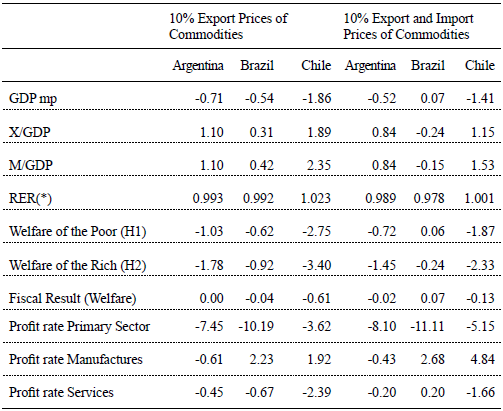
Tables 6 and 7 show the results of the shocks of export and import prices when it is assumed that the domestic mobility of capital is higher (25% and 50% from initial calibrated level of 12%). The degree of mobility of capital is a difficult parameter to be estimated, but it is relevant for the final results.
As can be seen in the Tables, the impact of the fall of prices is less significant when capital can be allocated more easily between production sectors. The differential results are more important for Argentina and Brazil, and less relevant for Chile.
Table 7. Results under real wages inflexibility and capital mobility of 50% (% of change).
(*) Level with respect to benchmark = 1. Source: own elaboration.
It can also be seen that the Fiscal Result is improved with capital mobility. Tokarick (1994) developed a CGE for Trinidad and Tobago to explore how the economies respond to trade liberalization and changes in terms of trade. He put emphasis on the fiscal result, and explored the implications of assuming compensatory adjustment in taxes. His model assumes that capital is specific and, therefore, equivalent to 0% mobility in our model. This should not be unexpected, since the economy implicitly increases resilience when a constraint (capital immobility) is relaxed.
The capital mobility could be the result of physical properties of assets, but also of macro or microeconomic policies aimed at compensating the negative shocks.
De Gregorio and Labbé (2011) pointed out that good fiscal management can compensate for negative shocks, but they referred mainly to inflation targeting and the use of the exchange rate. One additional result of our model is that the social or political determination of wages, as well as the policies that help to reallocate resources could be also effective in reducing volatility.
Tables 6 and 7 show that a higher degree of capital mobility improves the results for the three countries, but the effects are different. For the export prices simulation, we observe an improvement about 0.08 of GDP in Chile, 0.22 in Brazil and 0.45 for Argentina. These are a consequence of the different productive structure. In the case of import and export prices, the smallest effect is for Brazil (0.22), followed by Chile (0.35) and Argentina (0.61).
2. International Prices and full employment assumption
Table (8) shows the results under full employment. This is a counterfactual case since the three economies had positive unemployment for the benchmark year, though in the case of Chile, the levels of unemployment were close to the natural rate. Under full employment, the minimum nominal or real wage condition does not apply and the adjustment of wages responds to the interactions of demand and supply of labor. Surprisingly, the results do not look so different from those already obtained. One interesting thing to observe is that when export prices are lessened, the reduction of GDP is smaller, which indicates that the operation of the wage constraint was amplifying the shock. However, when import prices are reduced, the positive increase of the GDP of Brazil is also diminished.This indicates that increasing wages are growing and putting a limit to the expansion of the economy.
Table 8. Results under full employment (% of change)
(*) Level with respect to benchmark = 1. Source: own elaboration.
LESSONS AND CONCLUDING REMARKS
In this paper, we studied the vulnerability of three Latin American economies, Argentina, Chile and Brazil, to reductions of prices of exports of commodities, and how they could take advantage of reduction of imports of commodities.
Thus, we addressed five questions: (i) How will the economies react to a reduction of international prices of commodities?, (ii) How will the results change to a similar reduction of prices of imports?, (iii) Does the response depend on the capital/labor ratio?, (iv) Will there be relevant differences when wages are adjusted in real or nominal terms?, (v) Will the mobility of capital be relevant for the results?
To answer them and to appraise the full effect of the external shock, we constructed three CGE models. These models show how the determination of prices impacts on the remuneration of factors and consequently on income of households and on the fiscal result.
We found that the macroeconomic performance, income distribution and welfare of the economies depend on four basic parameters of the economies: the share of exports in GDP, the share of exports of commodities in exports, the import-intensity of manufactures and the share of labor in GDP.
The results of the simulations show that the economy of Argentina is vulnerable to the reduction of prices of commodities because it is dependent on exports of agricultural commodities or their derivatives (like soybean and soybean oil). Moreover, downward inflexibility of nominal wages can amplify the shock, because the economy is labor-intensive. Chile is vulnerable to price reductions because it is highly dependent on prices of copper and because it does take advantage of import prices reductions to a limited extent. However, Chile has developed contingent funds and its economy is less labor-intensive. Brazil would be the less affected by falls of commodities prices because its economy is more diversified and the manufacturing sector could be benefitted by reductions of prices of imported inputs. Thus, the opposite conclusion applies for Brazil: an increase of prices of imported commodities could have a negative impact on the economy.
The volatility of GDP depends on the degree of mobility of capital between production sectors too. This could support the idea that not only good macroeconomic policies could help to overcome negative shocks, but also the regulatory and institutional environment could be relevant.
We left two additional questions for future research: (i) Will the international mobility of capital be a key variable for the results?, (ii) Is it possible to compensate the impact on growth with tax instruments or contingency funds?
The first question seems of great interest, because the exit of capital to the rest of the world could exacerbate the vulnerability; this is explored by Céspedes and Velasco (2012). The second question focuses on good management of fiscal policy and the resources obtained in times of bonanza to compensate periods of scarcity, which is exemplified by the case of Chile (see De Gregorio (2012)).
Appendix Table 1 The Social Accounting Matrices
Notas
° Chisari, O., Mastronardi, L. J., & Romero, C. (2019). Commodities prices and critical parameters for macroeconomic performance: a CGE analysis for Argentina, Brazil and Chile. Estudios económicos, 36(72), 5-30
1 Alam et al. (2016), Fan et al. (2007) and Ganguly et al. (2016) are examples of the usage of CGE models to study the impact from international prices in a national economy structure.
2 The solution of the model is obtained using the representation of General Equilibrium and the Mixed Complementarities Approach. The model is developed in the environment of GAMS/MPSGE. At present, it can be used in interface with GAMS.
3 The models are equivalent, but they have a different sectoral disaggregation as a consequence of different country specific commodities and troubles in data collection. Argentine SAM was built for 2006 and it has 6 sectors: Primary sector; Mining and petroleum; Manufactures; Electricity, gas and water; Transport and Other services. Brazilian SAM was built for 2008 and it has 12 sectors divided into Agriculture; Forestry; Mining; Intensive industry energy use; Rest of manufactures; Oil refining; Electricity, gas and water; Construction; Trade; Transport and Other services. Chilean SAM was built also for 2008 and it has 7 sectors divided into Primary sector; Mining and petroleum; Chemical, paper and plastics; Rest of manufactures; Electricity, gas and water; Transport and Other services. A summary of each SAM can be consulted on Annex I.
4 For simulations, P* and Pm represent the subset of export and import commodities, respectively.
REFERENCES
1. Alam, M. J., Buysse, J., Begum, I. A., Nolte, S., Wailes, E. J., & Van Huylenbroeck, G. (2016). Impact of trade liberalization and world price changes in Bangladesh: a computable general equilibrium analysis. Agricultural and Food Economics, 4(1).
2. Banco Central de Chile. (2009). Cuentas Nacionales de Chile 2003-2009. Santiago: Banco Central de Chile.
3. Banco Central de Chile. (1996). Matriz de Insumo-Producto de la Economía Chilena 1996. Santiago: Banco Central de Chile. Recuperado de https://si3.bcentral.cl/estadisticas/principal1/informes/ccnn/cdr/matriz1996.pdf
4. Bonari, D., & Gasparini, L. (2002). El impacto distributivo de la política social en la argentina: Análisis basado en la encuesta nacional de gastos de los hogares. (Dirección de Gastos Sociales Consolidados, Ministerio de Economía. Serie gasto público, Documento de trabajo No. 12). Recuperado de https://www.economia.gob.ar/peconomica/basehome/impacto2002.pdf.
5. Bugarin, M. S., Ellery Jr, R., Gomes, V., & Teixeira, A. (2002). The Brazilian depression in the 1980s and 1990s. Recuperado de https://www.researchgate.net/profile/Roberto_Jr2/publication/24127898_The_Brazilian_Depression_in_the_1980s_and_1990s/links/0f31753b8ced9e56b6000000/The-Brazilian-Depression-in-the-1980s-and-1990s.pdf
6. Cattaneo, A. (2002). Balancing agricultural development and deforestation in the Brazilian Amazon. (IFPRI Research Report No. 129). Recuperado de https://ageconsearch.umn.edu/bitstream/16533/1/rr020129.pdf
7. Céspedes, L. F., & Velasco, A. (2012). Macroeconomic performance during commodity price booms and busts. IMF Economic Review, 60(4), 570-599.
8. Chisari, O. O., Estache, A., & Romero, C. A. (1997). Winners and losers from utility privatization in Argentina: lessons from a general equilibrium model. (Policy Research Working Paper No. 1824). Washington: World Bank Publications.
9. Chisari, O., Romero, C., Ferro, G., Theller, R., Cicowiez, M., Ferraro, J., ... & Maquieyra, J. (2009). Un modelo de equilibrio general computable para la Argentina. Buenos Aires: Programa de las Naciones Unidas para el Desarrollo.
10. Chisari, O. O., Maquieyra, J., & Miller, S. J. (2012). Manual sobre Modelos de Equilibrio General Computado para economías de LAC con énfasis en el análisis económico del Cambio Climático. Washington D. C.: Banco Interamericano de Desarrollo.
11. Chisari, O. O., Estache, A., Lambardi, G. D., & Romero, C. A. (2013). The trade balance effects of infrastructure services regulation. International Economics and Economic Policy, 10(2), 183-200.
12. De Gregorio, J. (2012). Commodity prices, monetary policy, and inflation. IMF Economic Review, 60(4), 600-633.
13. De Gregorio, J., & Labbé, F. (2011). Copper, the real exchange rate and macroeconomic fluctuations in Chile. (Banco Central de Chile, Documentos de Trabajo No. 640). Recuperado de http://si2.bcentral.cl/public/pdf/documentos-trabajo/pdf/dtbc640.pdf
14. Ellery Jr, R., Gomes, V., & Sachsida, A. (2002). Business cycle fluctuations in Brazil. Revista Brasileira de Economia, 56(2), 269-308.
15. Fan, Y., Jiao, J., Liang, Q., Han, Z. Y., & Wei, Y. (2007). The impact of rising international crude oil price on China's economy: an empirical analysis with CGE model. International Journal of Global Energy Issues, 27(4), 404-424.
16. Ganguly, A., & Das, K. (2016). Impacts of Falling Crude Oil Prices and Reduction of Energy Subsidies on the Indian Economy: A CGE Modelling Approach. Vision, 20(4), 345-360.
17. Gomes, V., Bugarin, M. N., & Ellery-Jr, R. (2005). Long-run implications of the Brazilian capital stock and income estimates. Brazilian review of econometrics, 25(1), 67-88.
18. Guilhoto, J. J. M., & Sesso Filho, U. A. (2005). Estimação da Matriz Insumo-Produto a Partir De Dados Preliminares das Contas Nacionais. Economia Aplicada, 9(2), 277-299.
19. Instituto Brasileiro de Geografia e Estatística (2004). Sistemas de Contas Nacionais. (IBGE Séries Relátorios Metodológicos No. 24. Recuperado de https://biblioteca.ibge.gov.br/visualizacao/livros/liv3942.pdf
20. Instituto Brasileiro de Geografia e Estatística (2007). Sistemas de Contas Nacionais - Brasil, Referência 2000. Notas Metodologias para nova série do Sistema de Contas Nacionais, referência 2000.
21. Lanteri, L. N. (2009). Términos de intercambio externos y balanza comercial: Alguna evidencia para la economía argentina. Economía mexicana. Nueva época, 18(2), 221-247.
22. Montero, R. (2005). Chile: Social Accounting Matrix, 1996. Washington, D. C.: International Food Policy Research Institute (IFPRI).
23. Ministerio de Ciencia y Tecnología (2010). Second National Communication of Brazil to the United Nations Framework Convention on Climate Change.
24. Rossignolo, D. (2003). El Federalismo Fiscal y la distribución personal del ingreso. Una medición preliminar para 2002. Publicado en los Anales de la XXXVIII Reunión Anual de la Asociación Argentina de Economía Política, Buenos Aires.
25. Rossignolo, D. A., & Santiere, J. J. (2001). Medición de la incidencia del sistema impositivo sobre la distribución del ingreso. Publicado en los Anales de la XXXV Reunión Anual del la Asociación Argentina de Economía Política, Buenos Aires.
26. Santiere, J. J., Gómez Sabaini, J. C., & Rossignolo, D. (2000). Impacto de los impuestos sobre la distribución del ingreso en Argentina en 1997. Buenos Aires: Banco Mundial, SPEyR, Ministerio de Economía.
27. Tokarick, S. (1995). External shocks, the real exchange rate, and tax policy. Staff Papers, 42(1), 49-79.
© 2019 por los autores; licencia otorgada a la Revista Estudios Económicos. Este artículo es de acceso abierto y distribuido bajo los términos y condiciones de una licencia Atribución-No Comercial 3.0 Unported (CC BY-NC 3.0) de Creative Commons. Para ver una copia de esta licencia, visite http://creativecommons.org/licenses/by-nc/3.0/


