


Servicios Personalizados
Articulo
 pdf en Español
 Articulo en XML
 Referencias del artículo
 Permalink
Latin American applied research
versión On-line ISSN 1851-8796
Lat. Am. appl. res. vol.42 no.1 Bahía Blanca ene. 2012
A Numerical method for the solution of confined co-flowing jet diffusion flames
G. S. Lorenzzetti†, A. L. De Bortolo‡ and L. D. F. Marczak†
†Graduate Program in Chemical Engineering, UFRGS, Porto Alegre, Brazil
greice.lorenzzetti@ufrgs.br, ligia@enq.ufrgs.bt
‡Graduate Program in Applied Mathematics, UFRGS, Porto Alegre, Brazil
dbortoli@mat.ufrgs.br
Abstract— The aim of this work is the development of a method to obtain the shear layer, which appears in confined co-flowing jet diffusion flames. A convenient formulation, based on the mixture fraction for fluid flow and on flamelet models for the chemistry, using the RANS (Reynolds Averaged Navier-Stokes) and the LES (Large Eddy Simulation) approaches, is chosen. Numerical tests, for the governing equations discretized using the second order finite difference explicit scheme, were carried out for Sandia Flame D to compare the results with data in the literature. Results of the shear layer development comproves the ability of the developed LES method solving diffusion flames.
Keywords— Diffusion Flames; Co-Flowing Jet; Methane; Finite Difference; Low Mach-Number.
I. INTRODUCTION
The field of combustion requires studies in thermodynamics, chemical kinetics, fluid mechanics, heat and mass transfer, turbulence, among others areas (Kuo, 2005). The combustion not only generates heat, which can be converted into power, but also produces pollutants such as oxides of nitrogen, soot, and unburnt hydrocarbons. In addition, unavoidable emissions of CO2 are believed to contribute to the global warming. These emissions will be reduced by improving the efficiency of the combustion process, thereby increasing fuel economy (Peters, 2000).
In gaseous turbulent combustion, the mixing processes can be divided into premixed, nonpremixed, or partially premixed. In this paper we work with nonpremixed combustion, where the fuel and the oxidizer enter separately the combustion chamber.
For many turbulent diffusion flames, the so-called flamelet concept can be used. The flamelet model describes a turbulent flame as a laminar flame in a turbulent flow field. There is general agreement that the flamelet concept is applicable in the zone of large Damkohler numbers with turbulent scales larger than the flame thickness (Warnatz et al., 2001).
The low Mach-number method is employed because usually the combustion occurs in this flow regime. For example, most of the accidental fire problems such as forest fires, fires in road tunnels and fires in buildings, arise at low Mach-numbers, where the local flow velocities are well below the local speed of sound. In addition, combustion within industrial burners normally occurs at low Mach-numbers. For these applications an approach that takes into account the compressibility is necessary (Howard and Toporov, 2007). When the Mach-number goes to zero the pressure gradient contribution in the nondimensional momentum equations becomes singular. Therefore, a numerical method used to integrate the original set of equations tends to fail when applied to very low Mach-numbers in combustion (Klein, 2001).
The combustion involves a large range of time and length scales that are originated from the heat release due to chemical reactions, which induce to strong con-vective, diffusive and radiative heat transfer. The complexity of the Navier-Stokes equations turns the Direct Numerical Simulation (DNS) of turbulence difficult for most flows of interest, because the number of degrees of freedom grows faster than 0(Re11/4) [0(Re9/4) in space and O (Re1/2) in time], where Re denotes the turbulent Reynolds number (Garnier et al., 2009). For the simulation of turbulent combustion the Reynolds Averaged Navier-Stokes (RANS) and the Large Eddy Simulation (LES) turn alternatives.
In this context, the present work is based on the mixture fraction for fluid flow and on flamelet models for the chemistry. We show some inedit numerical results of the shear layer development for a confined co-flowing jet of methane obtained using a finite difference scheme for the discretization of the governing equations. The dynamic pressure gradients come from a Poisson's equation scaled by the Mach-number. The model is validated through comparison with experimental data.
II. MODEL FORMULATION
A convenient formulation for nonpremixed flames, based on the mixture fraction for fluid flow (Bilger, 1980) and on flamelet models for chemistry, is chosen. The flamelet concept assumes that a small instantaneous flame element embedded in a turbulent flow has a structure of a laminar flame (Peters, 2000). The flamelet equations describe the balance among the unsteady changes, the diffusive effects and the chemical reactions.
Consider the following one-step reaction
 (1) (1) |
In a stoichiometric mixture, the fuel and the oxygen are entirely consumed after combustion to form CO2 and H20.
The set of governing equations includes the momentum, mixture fraction, energy and species mass fraction. Contribution arising from radiation is considered negligible in this formulation, since it is more important for large flames as in furnaces, spreading of fires in buildings and forest fires (Law, 1984).
When using Reynolds-aver aged approaches to model turbulence, all of the unsteadiness is averaged out, that is, all unsteadiness is regarded as part of the turbulence. On averaging, the non-linearity of the Navier-Stokes equations gives rise to terms that must be modeled (Ferziger and Peric, 2002). We employ the eddy-viscosity model for the Reynolds stress 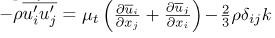 and the eddy-diffusion model for the mixture fraction
 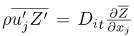 , where ρ is the density, uj the velocity vector, Z the mixture fraction (0 < Z < 1), μt the eddy viscosity, Dit the mass diffusivity of each species i in the turbulent condition, and k the kinetic energy.
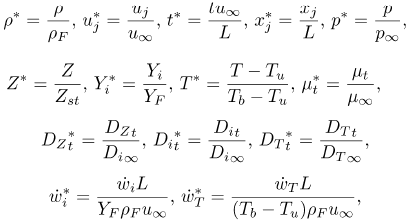
The set of governing equations may be conveniently written in nondimensional form if the following nondi-mensional quantities are defined:
 (2) (2) |
where the subscript ∞ refers to the conditions in the ambient air, F in the fuel, μ in the unburnt state, b in the burnt state, t in the turbulent condition, and st in the stoichiometric condition; L is a reference length, t the time, p the pressure, Yi the mass fraction of each species i, T the temperature, DZ the mixture fraction diffusivity, DT the thermal diffusivity,  the chemical source term, and
  the heat release rate.
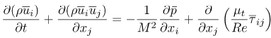
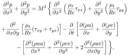
The Reynolds-averaged Navier-Stokes equations in nondimensionalised form, omitting the  are given by
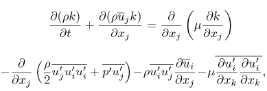
Momentum
 (3) (3) |
Mixture fraction
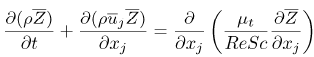 (4) (4) |
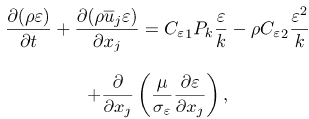
Energy
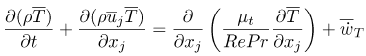 (5) (5) |
Species mass fraction
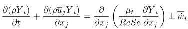 (6) (6) |
Here, τij is the resolved viscous stress tensor whose components are τxx, τxi, τxy, τyx and τyy.
The equation for  , where is a space and time function, does not contain any source term, since represents the initially chemical elements contained in the fuel; they are conserved during combustion. The mixture fraction measures the reactants mixing and is mainly related to the large scale motions of the flow. In these equations M is the Mach, Re the Reynolds, Sc the Schmidt, and Pr the Prandtl number.
The turbulent viscosity is modeled as (Peters, 2000; Warnatz et al, 2001)
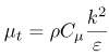 | (7) |
where Cμ is a constant and ε the dissipation. The k - ε model is based on the equation
 (8) (8) |
and
 (9) (9) |
where 
 (Ferziger and Peric, 2002).
As the flamelets are associated with the reaction zone, which is located in the vicinity of the stoichiometric mixture, the instantaneous local velocity of a flamelet particle has to be associated with the velocity of a point on the surface of a stoichiometric mixture fraction. After employing appropriate transformations (Peters, 2000; Pitsch and Steiner, 2000) results the known unsteady flamelet equations
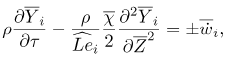 (10) (10) |
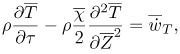 (11) (11) |
where τ is the time defined in the coordinate system attached to the stoichiometric surface, and  is the scalar dissipation rate given by
 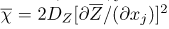 .
.  is defined as
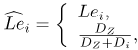 | in laminar flow regions, in turbulent flow regions, | (12) |
where Lei is the Lewis number of each species which is assumed to be equal to one in this paper. If the scalar dissipation rate changes rapidly, the unsteady term in the flamelet equations must be retained leading to a slow relaxation of the profiles (Peters, 2000).
For the simulation of diffusion flames, the method for low Mach-number seems to be appropriate. In this formulation, density comes from the state relation and it is necessary to write an equation to obtain the pressure gradients needed to correct the velocities. The pressure gradient is obtained after solving a Poisson's equation for pressure satisfying
 (13) (13) |
Note that the dynamic pressure is very small (less than 0.01% of the total pressure) and the corresponding pressure gradients are even smaller. The RHS (right hand side) of pressure equation is multiplied by M2, that for small Mach implies in small values for the pressure.
The space discretization follows the second order finite difference scheme. Central schemes are preferred since they are not dissipative; such property is desired to avoid damping of the small scales of turbulence, which are important in reactive flows.
While in the RANS approach all the unsteadiness is averaged out, the LES simulations are 3D, time dependent, but less costly than the DNS simulations. LES is a multi-scalar representation used for the solution of transient and turbulent flows. Using LES, the model for the turbulent viscosity becomes less important the better the mesh resolution, although refining the grid is restricted due to the rapid increase of the computational cost. Since the turbulence affects the flow in profound ways, it is common to find significant differences between the DNS (Direct Numerical Simulation) and LES predictions. This leads to the possibility of using LES for coarse meshes as a tool for determining the gross features of the flow (Ferziger and Peric, 2002).
In the case of LES, the set of governing equations can be derived by applying a density weighted Favre filtering. We employ the large-eddy simulation technique with the Smagorinsky model for the turbulent viscosity. This model is popular due to its simple formulation, and the turbulent viscosity is modeled as
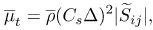 (14) (14) |
where  is the filter size,
 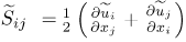 the rate of strain tensor and Cs the Smagorinsky coefficient. Satisfactory results are obtained with
  (Poinsot and Veynante, 2001).
III. NUMERICAL RESULTS
For the validation of the model it was chosen the Sandia flame D. Among the piloted flames, the flame D is preferred by several authors such as Barlow and Frank (2003), Pitsch and Steiner (2000), Schneider et al. (2003) and Sheikhi et al. (2005), because high Reynolds number is desired for model validation. Sandia flame D consists of a main jet with a mixture of 25% of methane and 75% of air. This jet is placed in a coflow of air and the flame is stabilized by a pilot. Figure 1 shows the fuel, and products CO2 and H2O mass fractions along the burner centerline for Sandia Flame D. These results are in good agreement with the experiment (Barlow and Frank, 2003).
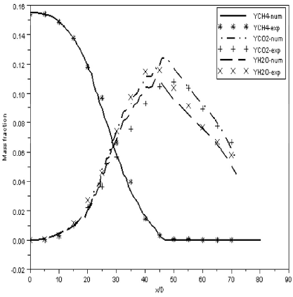
Figure 1: Comparison of the C/f4, COi and H2O mass fraction profiles along the burner centerline with the experiment (Barlow and Frank, 2003),
After checking the ability of an in house FORTRAN code solving jet diffusion flames, new results are obtained for the development of strong shear layers in jets. Therefore, consider the geometry of a two-dimensional channel with two splitter plates as shown in the Fig. 2. The configuration is a planar channel of streamwise length Lc in which three horizontal inlet streams of equal heights h/3 are separated by two splitter plates of equal length Ls to start mixing. The central stream velocity μi is varied relative to the two outer stream velocities μo to induce the development of the shear layer. The dimensions of the channel are h=3 0.06 m, Lc = 1.0 m, and Ls = 0.1 m.
Figure 2: Schematic of planar mixing in a symmetric channel.
We use a rectangular grid for the numerical simulations of the flame, with clustering close to the channel walls and splitter plate surfaces, to resolve the intricate details of the developing flow in the cross-stream direction, as shown in the Fig. 3. The mesh contains 1024 x 127 cells. At the inlet, three parabolic velocity profiles were provided for the three incoming streams, and the no-slip velocity condition was specified at all surfaces.
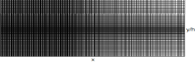
Figure 3: Mesh amplification, 1024x127 cells.
The unsteady flamelet equations are solved and the profiles showed are obtained after 1 second of simulation. The numerical simulations were performed using RANS, with the k â e model, and LES, with the Smagorinsky model. The equations with turbulence models are much stiffer than the laminar equations because the time scales associated with the turbulence are much shorter than those connected with the mean flow (Ferziger and Peric, 2002).
We compare here the results using RANS and LES to verify the differences between them for this two-dimensional problem, although the use of LES is appropriate in three-dimensions.
Figure 4 shows the instantaneous map of the mixture fraction, using RANS (left) and LES (right). The plots elucidate that fluid is entrained from the fast and slow feed streams into the shear layer. The developed code using LES capture the dynamical evolution of the mixing layer and the mechanisms of entrainment and mixing enhancement. The flow downstream of the plates is initially symmetric and eventually the wall effects break down the symmetry (Gokarn et a/., 2006). With RANS we observe a dissipation of the vortices; the unsteadiness effect is averaged out.
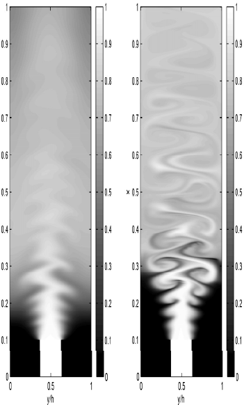
Figure 4: Mixture fraction map using RANS (left) and LES (right).
Figure 5 presents the mean profiles for velocity and mixture fraction obtained using LES, at different streamwise locations (x/Lc = 0.1; 0.3; 0.6; 0.8). It was observed that the higher the speed of the main jet, more developed turn the mean velocity profiles. This is due to the formation of a stronger shear layer, which reduces the velocity gradients between the central and co-flowing streams, thus, enhancing mixing.
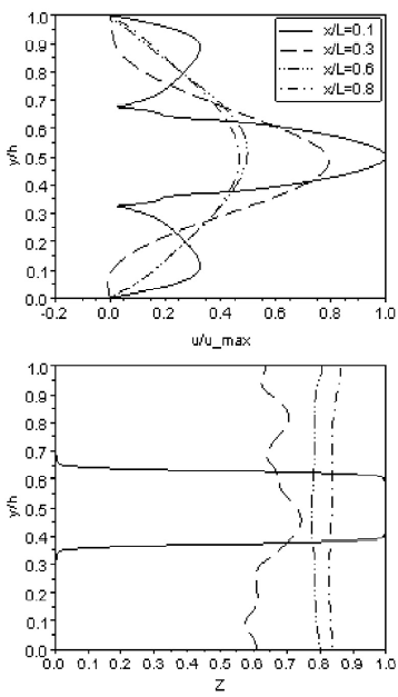
Figure 5: Normalized mean streamwise velocity (top) and mean mixture fraction (bottom).
The numerical results for the temperature, shown in Fig. 6, are in agreement with expectations, since the flamelet model assumes that the burning occurs in a thin layer of the flame, where we have a higher temperature. In the scale indicated in this figure, the value 1 corresponds to the ambient temperature and 8 to the highest flame temperature. Again in RANS we clearly observe the dissipative effect.
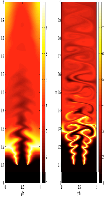
Figure 6: Temperature distribution inside the burner using RANS (left) and LES (right).
Finally, Fig. 7 shows the map for the product with RANS and LES. Note that the points of high temperature are those of highest concentrations of water vapor. This occurs because the products are formed in greater quantities where their mixture reaches the stoichiometric value. Our fluid flow results are in qualitative agreement with the works from Gokarn et al. (2006), Teleaga and Sea'id (2008) and Lawn (2009). Best results are obtained using LES, although its use is usually recommended only in three-dimensional simulations.
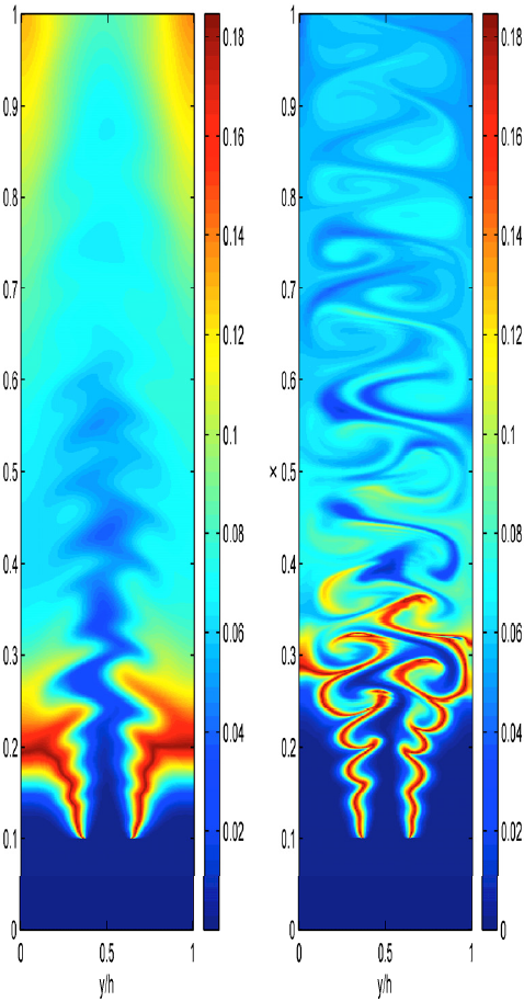
Figure 7: Instantaneous contour maps for the H2O mass fraction using RANS (left) and LES (right).
IV. CONCLUSIONS
This work developed a model to obtain the shear layer for co-flowing jet diffusion flames using the formulation of low Mach-numbers. The numerical results for mixture fraction, temperature, mass fraction of products, for a turbulent piloted methane-air jet diffusion flame, the Sandia Flame D, are in agreement with data in the literature.
The results of the development of the shear layer using LES contribute to a better understanding of the complexity involved in the numerical solution of jets mixing. The results for the flame in the development of this shear layer are inedit, and is one of the main contributions of the present paper. Our results for the fluid flow using LES, rather than RANS, compare better with the results of other authors found in the literature (Gokarn et al., 2006; Teleaga and Sea'id, 2008; Lawn, 2009) as by Ferziger and Peric (2002). Moreover, the good comparison between the numerical results and the experimental data, for Sandia Flame D, increase the reliability of the model proposed.
V. ACKNOWLEDGEMENTS
This research is being developed at UFRGS, Federal University of Rio Grande do Sul. The first author thanks the financial support from CAPES, Coor-denagao de Aperfeigoamento de Pessoal de Nwel Superior and the computational support from CESUP (Centro Nacional de Supercomputacao). The second author gratefully acknowledges the financial support from CNPq, Conselho Nacional de Desenvolvimento Cientifico e Tecnologico, under process 303007/20095.
REFERENCES
1. Barlow, R. and J. Frank, Piloted CPU/Air Flames C, D, E and F - Release 2.0, Consulted in: 25 October 2006, http://www.ca.sandia.gov/TNF(2003).
2. Bilger, R.W., "Turbulent Flows with Nonpremixed Reactants," in: Turbulent Reacting Flows, P. A. Libby and F. A. Williams, Eds., Springer-Verlag, Berlin, 65-113 (1980).
3. Ferziger, J.H. and M. Peric, Computational Methods for Fluid Dynamics, 3rd Edition, Springer (2002).
4. Garnier, E., N. Adams and P. Sagaut, Large Eddy Simulation for Compressible Flows, Springer (2009).
5. Gokarn, A., F. Battaglia, R.O. Fox and J.C. Hill, "Simulations of mixing for a confined co-flowing planar jet," Computers & Fluids, 35, 1228-1238 (2006).
6. Howard, R. and D. Toporov, The eddy dissipation combustion model developed for large eddy simulation, Consulted in: 30 March 2010, http://abc.ua.pt (2007).
7. Klein, R., Numerics in Combustion, Lecture Series of Von Karman Institute for Fluid Dynamics, Belgium (2001).
8. Kuo, K.K., Principles of Combustion, 2nd Edition, John Wiley & Sons, Inc., Hoboken, New Jersey (2005).
9. Law, C.K., "Heat and Mass Transfer in Combustion: Fundamental Concepts and Future Challenges," Progress in Energy and Combustion Science, 10, 295-318 (1984).
10. Lawn, C.J., "Lifted flames on fuel jets in co-flowing air," Progress in Energy and Combustion Science, 35, 1-30 (2009).
11. Peters, N., Turbulent Combustion, Cambridge University Press, Cambridge, UK (2000).
12. Pitsch, H. and H. Steiner, "Large-eddy simulation of a turbulent piloted methane/air diffusion flame (Sandia Flame D)," Physics of Fluids, 12, 10, 2541-2554 (2000).
13. Poinsot, T. and D. Veynante, Theoretical and Numerical Combustion, R. T. Edwards, Inc. (2001).
14. Schneider, Ch., A. Dreizler, J. Janicka and E.P. Hassel, "Flow field measurements of stable and locally extinguishing hydrocarbon-fuelled jet flames," Combustion and Flame, 135, 185-190 (2003).
15. Sheikhi, M.R.H., T.G. Drozda, P. Givi, F.A. Jaberi and S.B. Pope, "Large eddy simulation of a turbulent nonpremixed piloted methane jet flame (Sandia Flame D)," Proceedings of the Combustion Institute, 30, 549-556 (2005).
16. Teleaga, I. and M. Seaïd, "Simplified radiative models for low-Mach number reactive flows," Applied Mathematical Modelling, 32, 971991 (2008).
17. Warnatz, J., U. Maas and R.W. Dibble, Combustion: Physical and Chemical Fundamentals, Modeling and Simulation, Experiments, Pollutant Formation, 3rd Edition, Springer-Verlag (2001).
Received: August 23, 2010.
Accepted: March 29, 2011.
Recommended by Subject Editor Walter Ambrosini.
