Methodology based on SVD for control structure design

L.A. Alvarez^†§ and J. Espinosa^‡

National University of Colombia. Faculty of Mines. Cra 80 No 65 - 223 Medellín Colombia
^† Process and Energy School. luz@pqi.ep.usp.br
^‡ Electric and Control Engineering School. National University of Colombia. jjespino@unal.edu.co
^§ Present address: LSCP/CESQ Chemical Engineering Department, Polytechnic School. University of São Paulo. Av. Prof. Luciano Gualberto trav 3, 380. CEP 05508-900 São Paulo (SP) Brazil. Tel. +55-11 30912237. Fax. +55-11 38132380.

Abstract— This work presents a methodology for control structure design based on the Singular Value Decomposition (SVD) of the Hankel matrix, constructed from the observability and controllability matrices. A weight index is proposed as a measure of the impact of each input and output variable and, based on it, an input-output pairing selection is performed. The methodology is validated using the Tennessee Eastman process and the result is compared to the relative gain method in frequency.

Keywords— Control Structure Design; SVD; Hankel Matrix; Tennessee Eastman Process.

I. INTRODUCTION

The growing demand for optimal operation and effective use of energy and raw materials in chemical processes has generated a need to design processes with tighter integration. Materials recycle as well as energy exchange between the different process streams, modify the dynamic behavior of the process and make it more difficult to control. Until now, the vast majority of control studies have focused in controller design and little attention has been paid to control structures. The relationship between controlled, measured and manipulated variables and how to link these variables to form control loops in plants are problems that, in practice, are solved heuristically, because there is not enough solid theory. The main existing methods for control structure design are based in relative gains (Bristol, 1966) and singular value analysis (Skogestad and Postlethwaite, 1996). Although these methods are well grounded, the process system representation used does not take completely into account the dynamic behavior of the process. So, existing methods could indicate less appropriate control structures.

The objective of this work is to present the development of a methodology for control loop configuration, based on a singular value analysis of the Hankel matrix. In discrete time, that matrix represents the input-output behavior of the process and implicitly contains the dynamics, which makes it a very generic representation. The methodology is validated in the partially controlled Tennessee Eastman process (Larsson et al., 2001) in two levels: external and internal loops. At the external level the objective is to build master control loops with variables with strong interaction, and at the internal level local or slave control loops which are heuristically trivial.

In Section II, the existing tools for control structure design are presented and later, in Section III, the new methodology based on the Hankel matrix is proposed. Section IV describes the system used for methodology validation and in Section V the results of the validation are shown. Finally, Section VI shows the conclusions.

II. METHODS FOR CONTROL STRUCTURE DESIGN

This section discusses some existing methods for the control structure design (CSD).

A. Relative Gains

The method was originally proposed by Bristol (1966) and determines which variables are most convenient for pairing control loops in the process. Relative Gain Array (RGA) gives a measure of the interaction for each possible pairing. The original formulation uses the transfer function matrix of the process, evaluated at steady state, ignoring the dynamic behavior. In order to correct this and other limitations, several extensions have been proposed: RGA at Crossover frequency (Grosdidier et al., 1985), Relative gains for integrating processes (Arkun and Downs, 1990), RGA for non-square plants (Cao, 1995), RGA with operating frequency optimization (McAvoy et al., 2003), RGA integrating gains from zero to the frequency bandwidth (Xiong et al., 2005).

B. Singular Value Decomposition

SVD is a matrix factorization that allows the determination of the singular values of any matrix. Consider the complex matrix G, it can be decomposed as G = UΣV^T. The diagonal matrix Σ contains the singular values σ_i ordered from largest to smallest, and two matrices U y V that are orthonormal. In practical terms, when a process system is represented by G, it can be said that each singular value σ_i represents a mode i of operating the process and, according to this, the largest singular values indicate the most "energetic" modes. The vectors U_i of U and V_i of V represent the direction of each mode i. In that way the V_i indicate the direction of the process inputs and the U_i indicate de direction of the process outputs. This interpretation has generated the different CSD methods that use SVD as a tool. The CSD criteria are based in the maximum singular value, the condition number and the singular vectors:

- Maximum singular values: In general, it is desirable that the maximum singular value be small. In Havre et al. (1996) and Skogestad and Postlethwaite (1996) this index is used as a criterion for selecting secondary measurements, a SVD analysis of the transfer functions that relate the output error with the disturbance and the uncertainty is carried on. The idea is to maintain this value small for all the frequency range of interest.

- Minimum singular value: Morari (1983) argues that this value should be big in order for a plant to have a good tracking and regulation performance, in case of limitations in the magnitude of inputs. According to Skogestad and Postlethwaite (1996), by maintaining this value big, independent control of the variables can be guaranteed.

- Condition number (CN): This index is the ratio between the maximum and minimum singular value. The higher this value, the more difficult is the process control. A very high CN indicates that the plant tends to operate at certain modes and thus, the other modes would be difficult to attain. For this reason, a set of inputs and outputs that give a system with a small CN should be selected. Reeves (1991) proposed a method to reduce the number of candidate outputs and inputs. By calculating CN at crossover frequency some variables are eliminated gradually.

- Singular vectors: The methods based on the singular vectors U_i y V_i (Moore et al., 1987; Cao and Biss, 1996) try to weigh the effects of inputs and outputs to select input-output sets where control loops can be formed.

In brief, the methods here described are based on interaction and directionality. A possible drawback is the process representation, notice that these methods take the transfer function matrix G evaluated at steady state (G(0)) or at some relevant frequency, for example, the crossover frequency G(jω_C). For the steady state case, it is equivalent to suppose that the system always operates at steady state, disregarding system dynamics. When G is evaluated at a certain frequency, the process dynamics are "wrapped" at that frequency ignoring all other dynamics. The method proposed in this work aims to improve this point by using a discrete time domain representation of the system: the Hankel matrix.

III. SVD OF THE HANKEL MATRIX

The methodology presented here uses a system representation known as the Hankel matrix. From its singular value decomposition, a dynamical weighting of the effects of each input and output of the process is proposed. Using a selection criterion, input-output variable pairings for control loops are indicated.

A. Dynamic weighting of inputs and outputs

Consider a n^th-order system, with the following discrete state space representation:

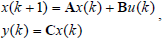(1)

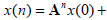
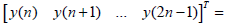
It is possible to determine the input-state and state-output relations. The observability matrix represents the relation between the initial state x(0) and the output measurement sequence y(0), y(1),... y(n-1):

(2)

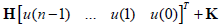
The controllability matrix represents the relation between the current state x(n) and a past sequence of inputs u(n-1)...u(1), u(0):

	(3)

Evaluating the Eq. 2 for the state in the n^th instant and replacing in the Eq. 3 an input-output expression is obtained:

	(4)

where H is Hankel matrix of the system and K is a constant:

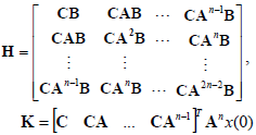Note that matrix H represents the input-output behavior of the system in dynamical terms, as it relates a sequence of inputs before the n^th instant with a sequence of outputs after the n^th instant. A SVD of H gives information about the dynamic impact of each variable in the system. In order to visualize the impact, a generic system with n=2 states, nu=3 inputs and ny=3 outputs was considered:

	(5)

Assuming that the system can be represented with the first singular value:

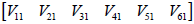	(6)

where U_ii are the components of vector U, V_ii the components of vector V and σ_i the singular values. Then, an output vector is obtained, expressed in terms of the components of the SVD matrices of H and the input sequence:

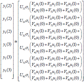(7)

From the eq. 7:

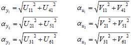(8)

where α_yi and α_uj measure the dynamic effect of the output i and input j respectively. Thus, in general terms, for a system with n states, nu inputs and ny outputs, if m singular values are taken, the impact on the output i and the impact of the input j are:

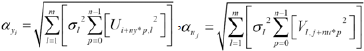(9)

B. Input-output pair selection criterion

Based on a singular value decomposition of G at steady state, Moore et al. (1987) proposed a selection of those inputs and outputs corresponding to the highest absolute values in the singular vector. The candidate variable set was intended to pair control loops. The method of Keller and Bonvin (1987) consists on selecting the set of inputs with the "strongest and most orthogonal effect" on the controlled outputs, this is quantified with the largest singular values and their corresponding singular vectors on matrix B from the state space plant description. Cao and Biss (1996) proposed a calculation of the "effectiveness" of each input using a SVD of G evaluated at the crossover frequency and with it, select the best set of inputs for process control.

This paper proposes the use of the weights in Eq. 9 to pair the inputs that have the largest impact with the most impacted outputs. These are the variables whose weights are the largest. When the control loop is selected, a new model is calculated for the system composed by the remaining variables (Eq. 1) and the process is repeated until all loops are closed. Figure 1 shows a schematic representation of the method.

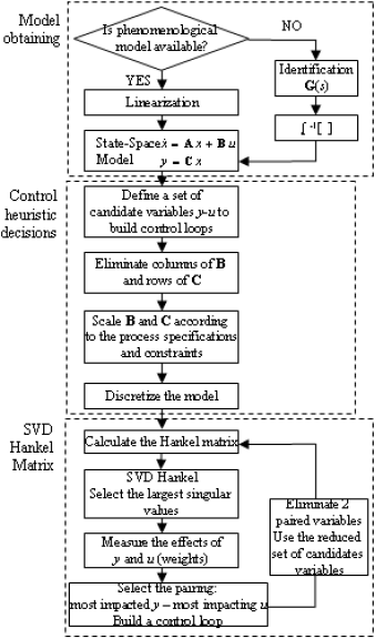
Figure 1. Schematic representation of the Hankel SVD methodology

IV. EXAMPLE: TENNESSEE EASTMAN PROCESS (TE)

Downs and Vogel (1993) published a model for an industrial chemical process from the Eastman Chemical Company, the model is now known as the Tennessee Eastman Process (TE). The purpose of the authors was to supply a benchmark problem to develop and evaluate different process control technologies. Figure 2 shows a simplified diagram of the TE process. This is composed of five operating units: reactor, condenser, liquid-vapor separator, recycle compressor and stripper column. The reactor is a two phase CSTR in which the products G and H are produced from reactants A, C, D and E. The process has 12 actuators and 41 measurements for control and monitoring. 22 of them are continuous while 19 are discrete. The operating point is defined as the mass relation between G and H in the product stream. Ricker (1995) identified the optimal steady state conditions for each of the operation modes. This article uses the 50/50 optimized mode. The measured and manipulated variable listing is omitted here, but can be found in Downs and Vogel (1993) or in Ricker (1995).

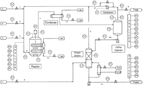
Figure 2. Tennessee Eastman Process Diagram

The methodology developed in this paper is not intended for unstable systems. As the TE process is open loop unstable, the process was stabilized with some control loops. So, the methodology was applied to the plant partially controlled. For this purpose an existent control structure was selected (Larsson et al., 2001). Some control loops were removed and the model was calculated for two different systems SI and SII, each one corresponds to a different hierarchical level. Both systems can be seen in Fig. 3. System SI contains variables of an external level, where dynamics have large interactions.

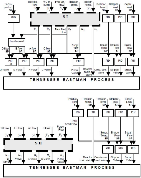
Figure 3. Systems SI and SII defined over the control structure from Larsson et al. (2001)

System SII contains variables of an internal level, where dynamics have small interactions and operate with a small time scale in comparison to the external level. Table 1 presents the variables for each system.

Table 1. Output and Input variables for systems SI and SII

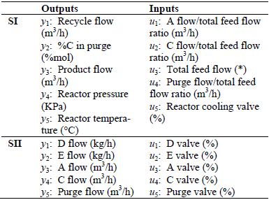
(*) adimensional.

Both SI and SII systems are stable when process is partially controlled. %G in product was not included in SI because that loop generates a more complex control structure that includes feedforward control and this uses another variable to control two variables.

Simulations were developed in Matlab 7.0. The TE process model used was implemented as a compiled S-function based in C code and the simulation environment used was Simulink. The plant model is continuous and the PID controllers are discrete. Before linearization, the equilibrium points were found numerically for each system. The TE plant in open loop has fifty continuous states and each discrete PID controller adds 2 states, in this case, discrete states. Because of this, the linear model of the plant was obtained using the small disturbance method and bilinear discretization. So a state space discrete model (Eq. 1) is calculated. For system SI a sample time of one hour was selected, this is the 1/20^th of the fastest dynamic of the plant: temperature y₅. Taking into account all states, continuous and discrete, system SI is of 74^th order and system SII of 66^th order. In order to validate the discrete models obtained, discrete linear models were compared with the original partially controlled plant models. By observing the response to a 3% step on all inputs, similar responses were found.

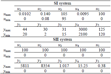
The input and output variables were normalized by defining them as the ratio between the variable and its variation interval, defined as the difference between the maximum and minimum values of the variable. This means that each element of matrix B should be divided by the input interval of that element and each element of matrix C by the output interval of each element. Maximum and minimum values for manipulated variables were taken from (Downs and Vogel, 1993). Maximum and minimum values for output variables were based on the desired process performance in agreement with the maximum and minimum expected variable values. These values are presented in Table 2.

Table 2. Maximum and minimum values for each input and output variables

V. RESULTS AND DISCUSSION

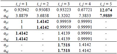
For both systems, the first five singular values of the Hankel matrix were taken, representing 99% of the "matrix energy" for SII and 95.53% for SI. The dynamic weights from the Hankel matrix SVD were calculated for SI and SII and are presented in Tables 3 and 4.

Table 3. Dynamic weights α_yi - α_uj in SI (External loops)

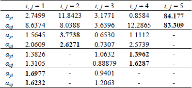
Table 4. Dynamic weights α_yi - α_uj in SII (Internal loops)

In SI the candidate variable set is composed by five inputs and five outputs. Notice that the most impacted output is y₅ the reactor temperature, and the input with the strongest impact is u₅, the opening of the reactor cooling valve. An y₅ - u₅ loop is paired. So, a new set with four inputs and four outputs remains and the Hankel matrix is again calculated. Here the most impacted output is y₂ (%C in purge) and the most impacting input is u₂ (C feed flow set point). A pairing with y₂ - u₂ is formed and a 3x3 system remains.

According to the impact indicated by the weights, a loop with y₄ - u₄ is paired, it suggests controlling the reactor pressure using purge flow set-point. With this loop closed, only two inputs and two outputs remain (y₁, y₃) and (u₁, u₃). For this subsystem y₁ (recycle flow) is the most impacted output and u₁ (A feed set-point) is the most impacting input. Thus y₁ - u₁ are paired. Finally y₃ and u₃ pair the last control loop, it means to control the production rate using the total feed flow as manipulated variable.

In SII, we deal with flow loops, whose pairing is heuristically trivial. Notice that in this case the most impacted output is y₅ and its weight is by far bigger than all of the output variables, which indicates that it is the most linked to the others and therefore the most impacted. The input with the strongest impact at this inner set is the purge flow valve u₅, so the loop y₅ - u₅ is paired. By eliminating these variables, the next candidate variables are all the feed flows, where heuristically is known that there is no interaction. In Table 4 it can be seen that for each flow-valve pair, the impact values are equal, which indicates that there is no interaction between the pairings. The other loops y₂ - u₂, y₁ - u₁, y₃ - u₃, and y₄ - u₄ were paired.

In order to compare the results presented here with a traditional method, the relative gain method was applied to the same systems SI and SII. The steady state gain matrix Λ is:

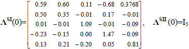For system SII, the relative gain array in steady-state is the identity matrix, so this method suggests the same pairings as the methodology presented here. However, in SI, the RGA method suggests pairing y₁ with u₂ and y₂ with u₁.

Now, to evaluate the results of the method extended to frequency analysis, which generates complex numbers, the real part of the relative gains and the distance from the desired complex value to 1+0i were plotted versus a frequency range. In Fig. 4, it is shown that, according to the relative gain method, pairing y₂ with u₂ is not convenient as the relative gain value deviates from desired complex value of 1+0i as frequency increases. However, Larsson et al. (2001) show that this configuration works and performs well and it is the same as indicated by the methodology here presented.

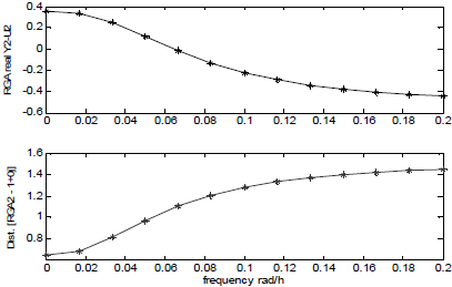
Figure 4. Relative Gain and distance from 1+0i in the full frequency range for y₂ - u₂ pair in SI

VI. CONCLUSIONS

The methodology presented in this paper is useful for designing feedback control structures with single loops. The main contribution of this method is an improvement compared with the relative gain and SVD based methods. In this case, the system representation captures the dynamic behavior of the process in the Hankel matrix, which is used for all the analysis. An index was proposed in order to measure the dynamic impact of the input and output variables and from this, a loop selection rule was formulated. When the methodology is applied to two subsystems defined in the TE partially controlled process, the results suggest a pairing already tested in simulation (Larsson et al., 2001). The method is also easy to understand and of direct use.

For system SII, composed by internal loops, pairings suggestion does not change when strongest loops are paired. This indicates that the pairing rule tends to work better when there is no interaction. It is also important to point out that the results vary significantly with process specifications, the minimum and maximum variable values, which are defined from heuristic process knowledge.

Finally, the method also has some limitations. First, it is restricted to stable systems. In order to extend the method to unstable systems, a stability analysis for each possible pairing should be included. Second, the systems defined to pair control loops must have dynamics at the same time scale. As the Hankel matrix represents the process dynamics directly, a system with dynamics at very different time scales would generate a Hankel matrix with poor information about the process, which would lead to wrong pairings.

ACKNOWLEDGMENTS
Financial support for this work was provided by Programa de Becas para Estudiantes Sobresalientes de Posgrado of National University of Colombia under grants: Res. 033/2006, 01/2007, 036/2007. J. Espinosa is also grateful to the HD-MPC of the European Union's seventh framework program, and Colciencias project 111845421919, CT-654-2008.

REFERENCES
1. Arkun, Y. and J. Downs, "A general method to calculate input-output gains and the relative gain array for integrating processes," Computers and Chemical Engineering, 14, 1101-1110 (1990).
2. Bristol, E.H., "On a new measure of interaction for multivariable process controlm" IEEE Trans. on automatic control, AC-11, 133-134 (1966).
3. Cao, Y., Control Structure Selection for Chemical Processes using Input-Output Controllability Analysis, PhD thesis. University of Exeter (1995).
4. Cao, Y. and D. Biss, "New screening techniques for choosing manipulated variables," Proceedings of IFAC World Congress, M, 103-108 (1996).
5. Downs, J.J. and E.F. Vogel, "A plant-wide industrial process control problem," Computers and Chemical Engineering, 17, 245-255 (1993).
6. Grosdidier, P., M. Morari and B.R. Holt, "Closed-loop properties from steady-state gain information," Ind. Eng. Chem. Fundam., 24, 221-235 (1985).
7. Havre, K., J. Morud and S Skogestad, "Selection of feedback variables for implementing optimizing control schemes," Proceedings of UKACC International Conference on Control, 1, 491-496 (1996).
8. Keller, J.P. and D. Bonvin, "Selection of inputs for the purpose of model reduction and controller design," Proceedings of IFAC World Congress, 209-214 (1987).
9. Larsson, T., K. Hestetun, E. Hovland and S. Skogestad, "Self-optimizing control of a large-scale plant: The Tennessee Eastman process," Industrial and Engineering Chemistry Research, 40, 4889-4901 (2001).
10. McAvoy, T.J., Y. Arkun, R. Chen, D. Robinson and P.D. Schnelle, "A new approach to defining a dynamic relative gain," Control Eng. Practice, 11, 907-914 (2003).
11. Moore, C., J. Hackney and D. Carter, "Selecting sensor location and type for multivariable processes," Proceedings of Shell Process Control Workshop, 291-308 (1987).
12. Morari, M., "Design of resilient processing plants III - a general framework for the assessment of dynamic resilience," Chemical Engineering Science, 38, 1881-1891 (1983).
13. Reeves, D.E., A comprehensive approach to control configuration design for complex systems, PhD thesis. Georgia Institute of Technology (1991).
14. Ricker, N.L., "Optimal steady-state operation of the Tennessee Eastman challenge process," Computers and Chemical Engineering, 19, 949-959 (1995).
15. Skogestad, S. and I. Postlethwaite, Multivariable Feedback Control, John Wiley & Sons (1996).
16. Xiong, Q., W. Cai and M. He, "A practical loop pairing criterion for multivariable processes," Journal of Process Control, 15, 741-747 (2005).

Received: October 20, 2010.
Accepted: October 2, 2011.
Recommended by subject editor: José Guivant