An augumented lagrangian method to solve three-dimensional nonlinear contact problems

F. J. Calavalieri and A. Cardona

Centro Internacional de Métodos Computacionales en Ingeniería CIMEC-INTEC (Universidad Nacional del Litoral -CONICET) Güemes 3450, S3000GLN Santa Fe, Argentina. fcavalieri@santafe-conicet.gob.ar

Abstract — A finite element formulation to deal with the friction contact problem between an elastic body and a rigid foundation is presented. An augmented Lagrangian method, which incorporates two Lagrange multipliers and a slack variable in the constraint equation, is developed. In this method, the solution is achieved through a Newton-Raphson monolithic iterative strategy and leads to simple implementation. Examples are provided to demonstrate the accuracy of the proposed algorithm.

Keywords — Contact; Augmented Lagrangian Method; Finite Elements; Friction.

I. INTRODUCTION

Nonlinear contact mechanics is used in many mechanical engineering branches, and numerous works have been dedicated to the numerical solution of contact problems, including the design of gears (Gamez-Montero et al., 2005), metal forming processes (Flores, 2000; Garino Garcia and Ponthot, 2008), contact fatigue (Madge et al., 2007) and many other applications. New advances and techniques, including friction, large deformation, plasticity and wear, are constantly being introduced. However, there is not yet a completely robust algorithm suitable for diferent applications in contact mechanics.

The governing equations for the contact problem are nonlinear and nondiferentiable; therefore, these equations pose severe convergence problems for the standard Newton-Raphson techniques. Several algorithms have been proposed in the literature to solve this problem. A complete review has been performed (Wriggers, 2002).

The penalty method is widely used in many contact algorithms. This method adds a "penalty" term to the energy functional, which regularizes the constraints. In this case, the displacement is the only primal variable in the formulation, and consequently, the computational implementation is relatively easy to be carried out. The disadvantage is that this method allows some penetration between the contacting bodies, and the user must choose a correct value of the parameter (the "penalty factor") in a rather arbitrary way to achieve acceptable solutions. The exact solution is obtained only for an infinite penalty value; however, a large penalty value leads to illconditioned matrices with severe precision losses in the computations. Therefore, many tests have to be carried out to find the correct penalty value and verify convergence.

Nonlinear contact mechanics can be related to nonlinear optimization problems, which allows the use of formulations with a more solid mathematical basis than the penalty method. The contact is modeled using inequality constraints. This problem can be formulated using the method of Lagrange multipliers, which results in a saddle point system to be solved at each iteration. An Uzawatype algorithm is often employed. In this double loop algorithm, the equilibrium problem is solved in the inner loop assuming a fxed value for the Lagrange multiplier. The Lagrange multipliers are then updated within the outer loop, and a new equilibrium problem is solved iteratively. This procedure finishes when the residual equilibrium, the residual constraints and the Karush-Kuhn-Tucker conditions are met within a certain tolerance. The method of Lagrange multipliers is very popular in contact mechanics because it overcomes the illconditioning inconvenience of the penalty method; however, it generates an increase in the matrix size due to Lagrange multipliers with null diagonal terms in the global stiffiness matrix, and this method results in a more complex implementation because of the double iteration strategy. If the problem is highly nonlinear, this procedure may be computationally expensive (Laursen and Maker, 1995).

A combination of both the penalty and the Lagrange multipliers techniques produces the socalled augmented Lagrangian method (Bertsekas, 1982). The augmented Lagrangian method was proposed frst by Hestenes (1969) and Powell (1969) to solve optimization problems with equality constraints. The addition of the penalty term to the Lagrangian constraints allows one to obtain a convex objective function far from the solution, which improves convergence. Both the augmented Lagrangian and the penalty methods require a penalty parameter. However, in the augmented Lagrangian method, the role of the penalty factor is only to improve the convergence rate, while in the penalty method, this factor determines the accuracy of the solution.

In frictional contact problems, when slip occurs, some numerical difculties arise due to the independence between the tangential force and the tangential displacement, which leads to a non-symmetrical stiffiness matrix. The friction phenomenon has been incorporated in the formulation of a unilateral contact by several authors; see, for example, Alart and Curnier (1991).

Several techniques have been proposed to incorporate the handling of inequality constraints in the Newton method, including the following examples: i) the active set strategies, which are applied in combination with the Lagrange multipliers (Hartmann and Ramm, 2008), ii) the use of slack variables on a slacked Lagrangian method (Byrd et al., 2000), and iii) the use of other techniques (Rockafellar, 1973; Tseng and Bertsekas, 1993). A Lagrangian method that used a combination of the Rockafellar Lagrangian method and an exponential Lagrange multipliers method together with a slack variable in the constraint was proposed by Areias et al. (2004).

In this work, which was inspired by the Lagrangian method presented in the paper of Areias et al. (2004), a new algorithm to solve contact frictional problems using an augmented Lagrangian method is presented. We modifed the activationjdesactivation conditions proposed by Areias et al. to solve the problem in a monolithic form using a Newton-Raphson strategy. This procedure avoids the use of the Uzawa algorithm and simplifes the practical implementation of the algorithm.

The work is organized as follows. Section II. describes the contact problem conditions. In Section III., the frictionless contact problem using Lagrange multipliers is presented and the matrices used to formulate the contact problem are detailed. Section IV.presents the friction contact problem. The algorithm for the solution of the frictional problem is described in Section V., where the stiffiness matrix related to the friction contact contribution is derived explicitly. In Section VI., two numerical examples are presented to demonstrate the performance of the proposed formulation, and conclusions are given in Section VII..

II. CONTACT PROBLEM DESCRIPTION

The equilibrium equation, in the context of a nonlinear problem and for a body β that occupies an open set Ω ⊆³with smooth boundary Γ, is given by the following equation

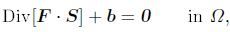(1)

where F , S, and b are the material deformation gradient, the second PiolaKirchhof stress tensor and the body forces in Ω, respectively. The second PiolaKirchhof stress tensor is related to the strains by an appropriate constitutive equation, i.e.,

S = C : E,

(2)

where C is the constitutive fourthorder tensor (Ogden, 1984), and E is the GreenLagrange strain tensor defined as

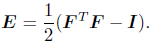(3)

In a general case, Signorini's contact problem consists of finding the elastic equilibrium confguration of an anisotropic, nonhomogeneous, elastic body resting on a rigid, frictionless surface. It is a boundary value problem where the displacement feld u has to satisfy the equilibrium equation as well as the Dirichlet, Neumann and contact conditions. In the case of the frictional contact, the problem becomes more complicated due to the nonconservative forces involved in the process.

Let us consider the body is supported by a frictionless, rigid foundation, as seen in Fig. 1. Then, Γ is split into three disjointed boundaries: Γu is where the body is fxed, Γσ is on which the surface traction is acting, and Γc is in contact with the rigid foundation. The boundary conditions are then expressed in the following form:

1. The Dirichlet boundary condition

(4)

2. The Neumann boundary condition

(5)

where t is the traction vector, F is the deformation gradient, N is the normal vector to the contact surface at the reference confguration and represents the prescribed traction vector.

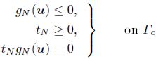
3. The contact conditions (Karush-Kuhn-Tucker Lagrange conditions)

(6)

where t_N = is the normal component of the traction vector, and (u) is the constraint function.

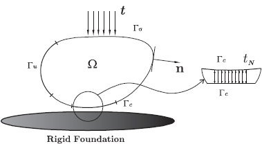
Figure 1: Contact between an elastic body and a rigid foundation.

In a contact mechanics framework, (u) represents the normal interpenetration function between bodies. The sign of indicates whether the bodies come into contact. A negative value implies that the bodies are not in contact, whereas a zero value indicates contact. Assuming, without loss of generality, that the contact surface is planar, i.e., normal contact, only the normal component of the traction vector t_N and the normal gap distance are taken into account.

For conciseness, this study is limited to the case of normal contact between the flexible body and a planar rigid foundation. This does not imply a lack of generality of the solution method, i.e., it can be extended to contacts between flexible bodies with any geometries; nevertheless, more elaborate methods need to be considered to model the geometric aspects and the interrelations between bodies.

III. FRICTIONLESS CONTACT ALGORITHM

The Finite Element Method (FEM) is used to discretize fexible bodies. Detailed FEM implementation descriptions for solid mechanics problems can be found in wellknown textbooks, e.g., Zienkiewicz and Taylor (2000); Bathe (1996); Crisfeld (2000). The fexiblejrigid contact problem using FEM can be formulated using

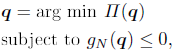(7)

where Π is the total potential energy, q is the global displacement vector, and (q) is the normal interpenetration evaluated at a given node. For simplicity, a simple nodal contact approach is used in this work. Nevertheless, the solution method can be applied with other techniques of modeling contacts, e.g., mortar methods (Wriggers, 2002). In the equations that follow, the contact at a single node is assumed to be a scalar function (q), but these equations can be directly extended to cases with vector nonlinear normal interpenetration functions.

The augmented Lagrangian for which stationary values are sought to solve problem (7) can be expressed as

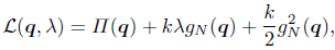(8)

where λ is the Lagrange multiplier and k is a scaling factor. Note that the scaling factor k times the Lagrange multiplier λ is equal to the contact normal force

(9)

because this term is conjugated to the normal interpenetration . The augmented Lagrangian method improves the convergence rate by adding convexity far from the solution with the penalty factor k (Géradin and Cardona, 2001). Usually, the augmented Lagrangian method needs to be combined with an Uzawa-type algorithm (Bertsekas, 1982). This is a double loop algorithm where, in the inner loop, the weak form of the equilibrium is solved with the set of active Lagrange multipliers held constant. Then, the sets of active Lagrange multipliers and inactive Lagrange multipliers are updated in the outer loop, the values of the active set are recalculated with displacements held constant, and the whole procedure is iterated until convergence is achieved in both cycles.

Instead of using this procedure, we propose to solve the contact problem and the weak form of the equilibrium at the same time using a standard Newton- Raphson iterative monolithic strategy. From Eq.(7), the inequality constraint can be transformed into an equality constraint and a side constraint by introducing the scalar variable s. In optimization theory, s is called a slack variable (Bauchau, 2000). By rewriting Eq.(7), the following system is obtained

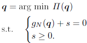(10)

In this way, the nonlinear inequality constraint has been replaced by an equality constraint and a simple linear side constraint, which acts directly on the newly added degree of freedom s. The augmented functional corresponding to Eq.(10), which includes the slack variable and a second Lagrange multiplier, takes the following form

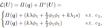(11)

where U = [q^T s λ λ1]^T, Π^c(U) is the contribution of contact to the system Lagrangian, the activationdeactivation conditions c₁ and c₂ are defined as

	contact,
	no contact,
	(12)

and where φ₁ is the slacked constraint:

(13)

The activation-deactivation conditions that are used here difer from the ones used in Areias et al. (2004).

Also, the expression of the Lagrangian used in Areias et al. (2004) was an exponential barrier, while here we are proposing to use a simple linear penalty, which we show give accurate results.

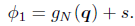
This formulation of the contact problem, in terms of an augmented Lagrangian with a slack variable and two multipliers, permits the use of a monolithic solution scheme based on the Newton-Raphson iterations for all of the variables simultaneously without an active set strategy. The solution to the contact problem is given by the set of values that render the augmented Lagrangian function stationary:

(14)

By taking variations in Eq.(11), we get the contributions of deformation energy and contact to the total virtual work:

(15)

where r (U) is the nonlinear residual vector:

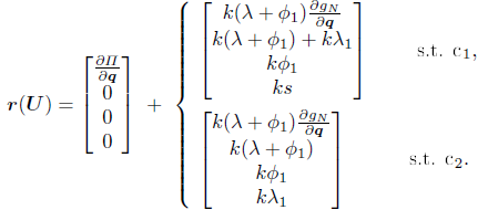(16)

Note that the fourth equation under condition c₂ is added to avoid having a singular system when the second constraint, corresponding to λ₁, is not active.

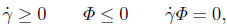
The latter system of equations can be differentiated to compute the contributions to the global stiffness matrix. These contributions take the following form:

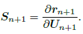
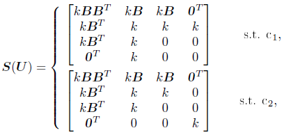(17)

where Β is the constraint gradients matrix Β = .

To describe the relative displacement between two contacting bodies, we adopt a node(slave)/surface (master) strategy where the contact normal force is evaluated at each active contact node of an element. Then, to compute the master surface normal vectors, the tangential vectors to the surface are required and are given by

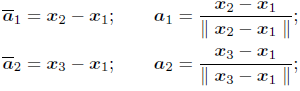(18)

where x_i represents the nodal coordinate vectors of the element contact surface, see Fig. 2. Then, the normal vector yields

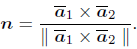(19)

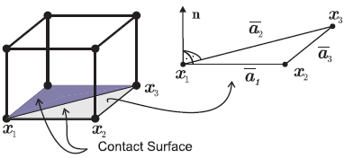
Figure 2: Regularization of the Coulomb law.

IV. FRICTIONAL CONTACT PROBLEM

The frictional contact problem is more cumbersome in its formulation and solution than the frictionless one. In the frictional contact problem, there are inequality constraints both in the normal and in the tangential directions at the contact interface. Two diferent states can now be distinguished: the "stick" state with null tangential displacement, and the "slip" state when tangential displacement occurs.

Some numerical difculties appear during the stick state. The Coulomb friction law imposes a null displacement, which corresponds to an infinite tangential stiffiness. To avoid this problem, a piecewise, linear regularized Coulomb friction law is used as shown in Fig. 3. This law assumes that, in the stick state, the tangential force depends linearly on the tangential displacement by a penalty factor (or tangential stiffiness) ε_T. This approach is physically justifed because the contact surfaces are not perfectly fat (Kikuchi and Oden, 1988). Based on this physical interpretation, other nonlinear formulations can be proposed. Usually, it is necessary to incorporate numerical parameters to adjust for the tribological behavior of the material (Kikuchi and Oden, 1988; Ling and Stolarski, 1997). However, the penalty parameter for the friction law has to be normally interpreted as a numerical coefficient.

Figure 3: Contact normal vector definition.

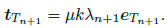
In the slip condition, the tangential force becomes independent from the tangential displacement, and is given instead by a relation with the normal contact force. For this reason, the stiffiness matrix becomes non-symmetric.

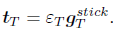
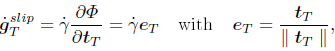
The equations for the frictional contact problem are derived by splitting the Cauchy traction vector t into a normal component t_N and a tangential component: t_T =(I − n ⊗ n)t. The total tangential displacement can be split into an "elastic" or stick portion and a "plastic" or slip portion ,

(20)

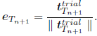
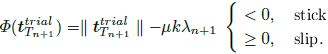
The state of sticking or slipping is recognized using the slip potential function Φ(t_T ):

(21)

where µ denotes the coefficient of friction. In case of having Φ(t_T ) < 0, the tangent contact force is less than µ times the normal contact force, and sticking occurs. When slipping, the tangent contact force equals the friction coefficient times the normal contact force, and the slip potential function is equal to zero. Note that the slip potential function should be strictly less than or equal to zero.

As mentioned before, a regularized Coulomb's law is used, see Fig. 3. In the pure stick case, the traction vector t_T is computed using an "elastic" constitutive law as follows,

(22)

Eq.(22) can be seen as a penalty regularization of the stick condition, = 0, with penalty constant ε_T . Slipping is formulated using an evolution law derived from the slip potential function Φ(tT ) (which is similar to the plastic potential in the framework of elastoplasticity). The constitutive equation for the slip path is

(23)

where is the unknown consistency parameter (slip rate). In the case of slipping, this parameter should be strictly positive; it is zero when the system is in stick condition.

Then, the Karush-Kuhn-Tucker conditions for frictional contact can be written as

(24)

where the last condition is the complementarity condition.

The frictional contact problem is therefore formulated by the set of equations for frictionless contact, i.e. Eqs.(16), supplemented with the Karush-Kuhn-Tucker conditions for frictional contact, Eqs.(24).

V. FRICTION ALGORITHM DESCRIPTION

There are many proposed algorithms to solve the friction problem (Simo and Laursen, 1992; Laursen, 1992; Alart and Curnier, 1991). In this work, an algorithm to update the tangential traction vector tT and the tangential displacement gT using an unconditionally stable backward-Euler integrator is used, which is also known as a return mapping algorithm. This algorithm is similar to that used for elastoplasticity (Simo and Hughes, 1998).

The contact virtual work expression, Eq.(15), is modifed by adding the contribution of the tangential friction forces as follows

(25)

where the terms δ and δg_T express the variations of the motion into directions normal and tangential to the contact surface Γ_c, respectively.

We assume the body slides on a rigid planar surface Γ_c to simplify the presentation. The relative tangential displacement at time t_n+1 can be expressed as

(26)

where t_v and t_w are two mutually orthogonal unit vectors tangent to the surface Γ_c, Δ_q is the increment of displacement, Fig. 4, and where

(27)

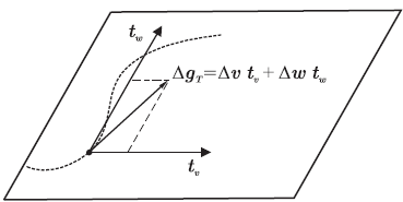
Figure 4: Tangential vector definition.

Assuming that the local state of the body at time t_n+1 is completely defined from the previous time t_n, the trial tangential force vector is defined as follows

(28)

where we have defined t_T = ε_T . The direction of the tangential force at time t_n+1 is coincident with the direction of the trial tangential vector

(29)

The slip potential function, Eq.(21), is evaluated for the trial state at the current time as

(30)

where t_N = kλ has been used, Eq.(9). In the case of sticking, there is no slipping component of motion, and the traction vector is equal to the trial force vector

(31)

while the tangential relative motion leads to

(32)

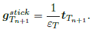
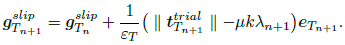
Otherwise, when slipping in the tangential direction occurs, we integrate Eq.(23) using a backward-Euler scheme to obtain:

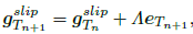(33)

where Λ = Δt denotes the unknown incremental slip. The traction vector is given by the expression:

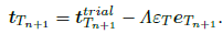(34)

Because we are in the slipping state, we set Φ =0 in Eq.(21), and by taking the norm of Eq.(34), we obtain Λ explicitly as follows

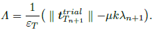(35)

Finally, with the incremental slip parameter Λ from Eq.(35), the traction vector t_{T n+1} and the tangential displacement vector g_{T n+1} at time t_n+1 are established by introducing Eq.(35) into Eq.(34) and Eq.(35) into Eq.(33). Thus,

(36)

(37)

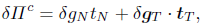
A detailed explanation of this algorithm can be found in Simo and Hughes (1998) or Wriggers et al. (2001). According to Eqs.(25,26), the contribution from the tangential friction term to the residual vector is given by

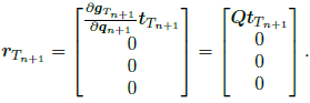(38)

The tangent matrix is obtained by differentiation of the residual force vector.

(39)

In the case of stick, the following form is obtained:

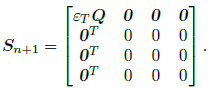(40)

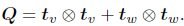
The procedure is analogous for the slipping state. The tangent matrix is calculated in this case as

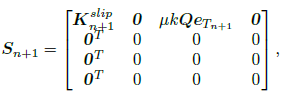(41)

where

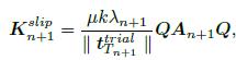(42)

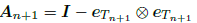(43)

VI. NUMERICAL EXAMPLES

Two numerical examples are presented to evaluate the robustness and accuracy of the proposed contact algorithm. The examples involve quasi-static simulations and were carried out in the research finite element code Oofelie (2011). All preand post-processing were perA detailed explanation of this algorithm can be formed using the software SAMCEF (2007).

A. Validation example I: 3D friction test.

This example represents an important validation test, tangential friction term to the residual vector is given which was originally presented by Oden and Pire (1984) as a 2D friction test, for the friction contact problem. More recent versions have been proposed by Armero and Petocz (1999) and Areias et al. (2004). Here, we compare our 3D results introducing a plane strain state, which reproduces the same 2D boundary conditions. The mesh topology, boundary conditions, dimensions and material properties are shown in Fig. 5.

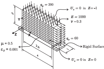
Figure 5: Elastic body pressed against a rigid foundation and pulled tangentially.

The material behaviour used in this example is linear elastic. The mesh has 462 nodes and 200 hexalinear finite elements as shown in Fig. 5. The lateral boundary conditions are used to reproduce the plane strain state. A uniform pressure q_y acts on the deformable body surface and presses it against the rigid foundation. Then, a horizontal pressure feld q_x, starting on one side of the body, pulls it. The final confguration is shown in Fig. 6. Figures 7 and 8 show the normal and tangential stress felds, respectively.

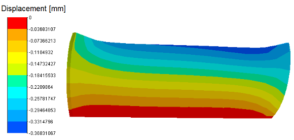
Figure 6: Final configuration. Displacement field in the Y direction.

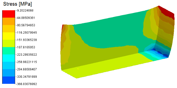
Figure 7: Normal stress field in the Y direction.

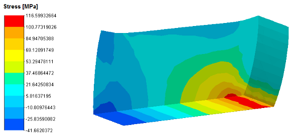
Figure 8: Tangential stress field in the X - Y direction.

Figure 9 shows a comparison of the results in terms of normal and tangential stresses. The results obtained agree with those obtained by Armero and Petocz (1999). These results were obtained in a single computational step with seven iterations.

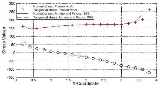
Figure 9: Normal stress σ_yy and tangential stress Γ_xy at the contact interface. The results are compared the results obtained by Armero and Petocz (1999).

B. Validation example II: 3D large displacements friction test.

This 3D friction example was proposed by Joli and Feng (2008). It consists of the contact analysis for a 3D cube on a rigid planar surface with a large amount of sliding.

Two prescribed displacements, α and b, are imposed at the top surface A-B-C-D as shown in Fig. 10. First, the vertical displacement a is applied and is followed by the horizontal displacement b with an orientation of 60° with respect to the X axis. The boundary conditions are summarized below

• Vertical displacement: α = (0, 0, −0.1) mm imposed in 10 equal load steps.
• Horizontal displacement: b = (0.4 cos 60, 0.4 sin 60, 0) mm imposed in 40 equal load steps
• Total number of load steps: 50.

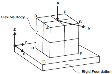
Figure 10: Cube on a frictional planar surface.

The elastic material property values are: E = 210000 N / mm² and ν =0.3, and the value for the coefficient of friction µ is 0.3. Each cube side length is 1 mm. The mesh has 27 nodes, with eight hexahedral nonlinear elements (see Fig. 10). The tangential stiffiness for the regularized Coulomb law is selected with a large value to reproduce the Coulomb law as accurately as possible (ε_T =5 × 10¹⁰).

A total of 50 computational steps are used in the simulation, giving with a mean of 7.3 iterations per step. The same problem was solved by Joli and Feng (2008), using a mean of more than 20 iterations per step. Fig. 11 shows the displacement components Ux and Uy at the point F, whereas Fig. 12 shows the normal contact force variation at the points F and H. Both curves agree with those presented by Joli and Feng (2008).

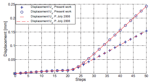
Figure 11: Displacement evolution U_x and U_y at the Applied Mechanics and Engineering, 179, 151-178

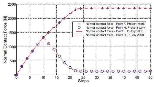
Figure 12: The normal force evolution at the points F and H. The results are compared with the results obtained by Joli and Feng (2008).

VIII. ACKNOWLEDGEMENTS
This work has received financial support from Agencia Nacional de Promoción Científca y Técnica (ANPCyT) and Consejo Nacional de Investigaciones Científcas y Técnicas (CONICET).

VII. CONCLUSION

A new contact algorithm using an augmented Lagrangian method with two Lagrange multipliers is proposed. The strategy of implementing an additional slack variable with a Newton-Raphson strategy in a monolithic scheme avoids the programming complications of algorithms based on activation j deactivation of constraints with a two-leveled iterative loop.

The strategy is based on a Rockafellar Lagrangian method and is similar to that presented in the work of Areias et al. (2004). Nevertheless, the approach presented here is simplified without using exponential barriers. Also, the conditions for activation / deactivation of constraints are different from those of Areias et al. (2004), and are implemented more easily.

The equations for the analytic computation of the residual forces and tangent matrices are presented. The strategy can be implemented very easily in a finite element program for nonlinear analysis without any change to the main structure of the code.

Two three-dimensional numerical examples with a frictional contact are shown. The results of these examples compared well with results from previous studies. The performance in the examples was good and demonstrates the potential of the proposed approach.

References
1. Alart, P. and A. Curnier, "A mixed formulation for frictional contact problems prone to Newton like solution methods," Comput. Methods Appl. Math., 92, 353-375 (1991).
2. Areias, P.M.A., J.M.A. César de Sá and C.A. Conceiçao António, "Algorithms for the analysis of 3D finite strain contact problems," International Journal for Numerical Methods in Engineering, 61, 1107-1151 (2004).
3. Armero, F. and E. Petocz, "A new dissipative timestepping algorithm for frictional contact problems: formulation and analysis," Computer Methods in Applied Mechanics and Engineering, 179, 151-178 (1999).
4. Bathe, K., Finite Elements Procedures, Prentice-Hall, Englewood Clifs, New Jersey (1996).
5. Bauchau, O.A., "Analysis of fexible multibody systems with intermitent contacts," Multibody System Dynamics, 4, 23-54 (2000).
6. Bertsekas, D.P., Constrained Optimization and Lagrange Multiplier Methods, Academic Press, New York (1982).
7. Byrd, R., J. Nocedel and R. Waltz, "Feasible interior methods using slacks for non-linear optimization", Optimization Technology Center, Otc 2000/11, Northwestern University, Evanston, IL, USA, February (2000).
8. Crisfeld, M., Non-linear Finite Element Analysis of Solids and Structures, 1, Wiley (2000).
9. Flores, F., "Un algoritmo de contacto para el análisis explícito de procesos de embutición," Métodos numéricos para el cálculo y diseño en ingeniería, 16, 421-432 (2000).
10. Gamez-Montero, P., F. Zárate, M. Sánchez, R. Castilla and E. Codina, "El problema del contacto en bombas de engranajes de perfl troncoidal," Métodos numéricos para el cálculo y diseño en ingeniería, 21, 213-229 (2005).
11. Garino Garcia, C. and J.P. Ponthot, "A quasicoulomb model for frictional contact interfaces. application to metal forming simulations," Latin American Applied Research, 38, 95-104 (2008).
12. Géradin, M. and A. Cardona, Flexible Multibody Dynamics. John Wiley and Sons (2001).
13. Hartmann, S. and E. Ramm, "A mortar based contact formulation fon nonlinear dynamics using dual lagrange multpliers," Finite Element and Design, 44, 245-258 (2008).
14. Hestenes, M., "Multiplier and gradient methods," J. Optim. Theory and Applic., 4, 303-320 (1969).
15. Joli, P. and Z.Q. Feng, "Usawa and Newton algorithms to solve frictional contact problems within the bipotential framework," International Journal for Numerical Methods in Engineering, 73, 317-330 (2008).
16. Kikuchi, N. and J. Oden, Contact Problems in Elasticity: A Study of variational Inequalities Constrains and Finite Element Method, SIAM, Philadelphia (1988).
17. Laursen, T., Formulation and treatment of frictional contact problems using finite element method, Phd thesis, Stanford Universtity, USA (1992).
18. Laursen, T. and B. Maker, "An augmented Lagrangian QuasiNewton solver for constrained nonlinear finite element applications," International Journal for Numerical Methods in Engineering, 38, 3571-3590 (1995).
19. Ling, W. and H. Stolarski, "A contact algorithm for problems involving quadrilateral approximation of surface," Comput. Struct., 63, 963-975 (1997).
20. Madge, J., S. Leen, I. McColl and P. Shipway, "Contactevolution based prediction of fretting fatigue life: Efect of slip amplitude," Wear, 262, 1159-1170 (2007).
21. Oden, J. and E. Pire, "Algorithms and numerical results for finite element approximation of contact problems with nonclassical friction laws," Computer and structures, 19, 137-147 (1984).
22. Ogden, R.W., Non-Linear Elastic Deformation, Dover Publications (1984).
23. Oofelie, Object oriented finite elements led by interactive executor, Open engineering S.A. Http://www.oofelie.org (2011).
24. Powell, M., "A method for nonlinear constraints in optimization," Optimization, R. Fletcher (Ed.), Academic, New York., 283-298 (1969).
25. Rockafellar, R., "A dual approach to solving nonlinear programming problems by unconstrained optimization," Mathematical Programming, 5, 354-373 (1973).
26. SAMCEF, Mecano V13 user manual. Samtech S.A. Http://www.samcef.com (2007).
27. Simo, J. and T. Laursen, "An augmented lagrangian treatment of contact problems involving friction," Computer and Structures, 42, 97-116 (1992).
28. Simo, J.C. and T.J.R. Hughes, Computational Inelasticity, Springer (1998).
29. Tseng, P. and D. Bertsekas, "On the convergence of the exponential multiplier method for convex programming," Mathematical Programming, 60, 1-19 (1993).
30. Wriggers, P., Computational Contact Mechanics, John Wiley and Sons (2002).
31. Wriggers, P., L. Krstulovic-Opara and J. Korelc, "Smooth C1interpolations for twodimensional frictional contact problems," International Journal for Numerical Methods in Engineering, 51, 1469-1495 (2001).
32. Zienkiewicz, O. and R. Taylor, The Finite Element Method, 2, Butterworth-Heinemann, Oxford, 5 edition (2000).

Received: May 24, 2011
Accepted: November 2, 2011
Recommended by subject editor: Adrian Lew