Improved neural network based CFAR detection for non homogeneous background and multiple target situations.

N.B. Gálvez^†, J.E. Cousseau^‡, J.L. Pasciaroni^† and O.E. Agamennoni^‡

^† SIAG-Servicio de Análisis Operativos, Armas y Guerra Electrónica Base Naval Puerto Belgrano -Av. Colón s/n - (8111) Punta Alta. Bs.As. E-mail: ngalvez@uns.edu.ar, pasciaro@uns.edu.ar
^‡ Instituto de Investigaciones en Ingeniería Eléctrica(IIIE) -Depto. de Ing. Eléctrica y de Computadoras. Universidad Nacional del Sur -Av. Alem 1253 -(8000)Bahía Blanca -Bs.As. jcousseau@uns.edu.ar, oagamen@uns.edu.ar

Abstract — The Neural Network Cell Average -Order Statistics Constant False Alarm Rate (NNCAOS CFAR) detector is presented in this work. NNCAOS CFAR is a combined detection methodology which uses the effectiveness of neural networks to search for non homogeneities like clutter banks and multiple targets within the radar return. In addition, the methodology proposed applies a convenient cell average (CA) or order statistics (OS) CFAR detector according to the context situation. Exhaustive analysis and comparisons show that NNCAOS CFAR has better performance than CA CFAR, OS CFAR and even CANN CFAR detectors (the latter, a previously proposed neural network based detector). Furthermore, it is verified that the new proposal presents a robust operation when maintaining a constant probability of false alarm under different radar return situations.

Keywords — Neural Networks; Threshold; CFAR; Clutter; Multiple Targets; Detection.

I. INTRODUCTION

In a previous work, the CANN CFAR was presented; it performs an homogeneity analysis of the radar return clutter by means of a neural network (NN). It was demonstrated that the NN homogeneity test has better performance when determining non homogeneities within a radar return than classical methods (Gálvez et al., 2011).

Some characteristics of classical CFAR algorithms are the following:

• The CA CFAR processor is the optimum CFAR processor (maximizes detection probability) in a homogeneous background for certain well defined conditions¹. As the size of the reference window increases, the detection probability approaches that of the optimum detector which is based on a fixed threshold (Gandhi and Kassam, 1988).
• The OS CFAR processor exhibits some loss of detection power in homogeneous noise background compared with the CA but its performance in a multiple target environment is clearly superior (Gandhi and Kassam, 1988).
• Multiple target situations, lead to almost negligible losses in OS CFAR processing compared with conventional CFAR processing (Rohling, 1983).
• The OS CFAR processor is unable to prevent excessive false alarm rate at clutter edges, unless the threshold estimate incorporates the ordered sample k near the maximum, that is unless k is very close to M; but in this case the processor suffers greater loss of detection performance (Gandhi and Kassam, 1988).

Gandhi and Kassam (1988) suggest that it may be interesting to consider adaptive versions of the OS schemes. For example, in the OS CFAR scheme, we may set the value of the kth sample adaptively based on some procedure that infers the background situation. This procedure will simply test whether the background is homogeneous or contains regions of clutter transitions (Gandhi and Kassam, 1988). The difficulty in finding one processing algorithm that accommodates the variety of environments encountered in practice has led to the development of composite processors (Smith and Varshney, 2000).

Taking advantage of the above classical CFAR characteristics, the NNCAOS CFAR offers the possibility of making an on line classification to each radar return by means of NN, with the purpose of applying the appropriate CFAR process over each range cell. This processor includes the same efficient NN block as the CANN CFAR (Gálvez et al., 2011) to estimate homogeneity in the case of clutter banks (CB), and incorporates an additional NN block to find out whether the radar return contains multiple targets (MT). These two NN blocks search for non homogeneities CB and MT within the radar return that allow to define suitable contexts for CFAR detection.

This work is organized as follows. In section II, some related basic detection models and notation are presented. The novel NNCAOS CFAR method is explained in Section III. A complete performance analysis, including simulation and comparisons, is presented in Section IV. Finally, the conclusions are expressed in Section V.

II. SOME BASIC CONCEPTS

In this section homogeneous and non homogeneous radar returns containing CB and MT are studied. A brief description of the model used, the Weibull radar return, is made. In addition, two classic CFAR detection schemes are reviewed: the OS and CA, where related threshold parameters, P_fa and P_d, are discussed. Considering the CFAR detection methodology to be described in the next section, a basic review of neural networks in this context is given in Gálvez et al. (2011).

A. Model Description

Because clutter is a random phenomenon, it is usually described in probabilistic terms, i.e. by a function of density of probability (pdf). In the last years, with the development of high resolution radars, it became evident that the clutter cannot always be modeled with a Gaussian distribution. The excessive increment in the amplitude of the waves, originating peaks in the distribution, surpasses the fixed threshold in the detection, causing an excessive number of false alarms. In recent investigations on sea clutter modeling, adaptive models have been used with other distributions such as Weibull, Rayleigh and K, which decrease the number of false detections. However, sea clutter constantly changes over time and none of the previous distributions can model it completely (López Estrada et al., 2004).

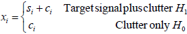
In that case, adaptive models have variable parameters that can be adjusted to the existing sea conditions (according, for example, to the Beaufort scale ²). In this way it is possible to associate an adaptive model to a group of sea states (López Estrada et al., 2004). Let x_i be an observation taken within some resolution cell i which represents a sampled radar return, observed over a time interval window (cell under test, CUT). The observation x_i may be composed by target s_i plus clutter c_i or clutter only, as given by

(1)

x_i may be considered to be a sampled function from one of two random processes. One is the sample of x_i under the condition that no signal is present H₀. The other, H₁, is the sample of x_i under the condition that both signal and clutter are present (Minkler and Minkler, 1990).

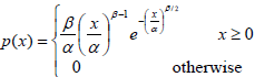
In this work the clutter is assumed to have Weibull distribution (Doyuran and Tanik, 2007) given by

(2)

where α is the scale parameter (indicating the energy level of the median) and Β is the shape parameter (indicating the degree of distribution skewness) (Minkler and Minkler, 1990). The Rayleigh distribution is a special case of the Weibull distribution with Β = 2. The mean value of the Weibull distribution varies according to the shape parameter, making it possible to describe range cells with values that can represent sea states of 1 to 3 (López Estrada et al., 2004).

The variability of the context of the radar return is modeled in this work considering two possible situations (sea conditions):

Case 1

Radar returns are modeled using (homogeneous) Weibull distribution according to Eq. (2) for different shape parameters (Β). The Weibull clutter model has been used to model both land and sea clutter and can generally be matched to experimental data over a much wider range of conditions than other distributions (as for example the log normal or Rayleigh models (Mahafza, 2000)).

Case 2

Radar returns are modeled using non homogeneous Weibull distribution, i.e. considering CB and MT. Clutter phenomena may be caused by a number of different sources. It may become necessary to identify clutter regions of differing clutter types and to describe their properties (in addition to type) such as size and borders, power and spectral features. The assumption of a uniform (homogeneous) clutter situation within the reference window is no longer maintained. Instead, provisions are made to handle transitions in clutter characteristics, clutter areas of small extensions, and interfering target echoes occurring within the reference window of the radar test cell (Rohling, 1983).

In this case, two specific situations are considered:

• Clutter banks (CB): In the case of non homogeneous returns, the clutter is assumed to have Weibull amplitude distribution and the distribution parameters change abruptly in range. A typical example of non homogeneous clutter return is illustrated in (Gálvez et al., 2011).
• Multiple targets (MT): This situation is presented when two or more closed useful targets are present in the CFAR window. Here a deterministic target model is preferred in order not to mix up the effects of mutual masking and of fluctuation (Rohling, 1983). In this case two situations are considered, a group of targets situated far away from clutter banks or a group of targets situated near the clutter bank. With many CFAR procedures, such a signal situation results in undesired effects such as masking of closely spaced targets (Rohling, 1983).

B. Conventional CFAR detection

A simplified CFAR detector is illustrated in Fig. 1. The CFAR detector can be described as a shift register with the radar return signal as the input. The amplitude in the CUT is compared to the CFAR detector output, scaled by δ (P_fa), the threshold multiplier, which is a scalar factor. The CFAR detector applies an algorithm to the M range cell values on both sides of the CUT. Immediate neighbouring cells are called buffer cells and are discarded to avoid contamination with the edge of the matched filter output from the target return (Rifkin, 1994). The detection threshold is computed so that the radar receiver maintains a constant pre-determined false alarm P_fa (Mahafza, 2000).

Figure 1: CFAR Scheme

The statistic Z, as depicted in Fig. 1, which is proportional to the estimate of total noise power, is formed by processing the contents of M reference cells surrounding the CUT whose content is X. A target is declared to be present if X exceeds the threshold T. Here T is a constant scale factor used to achieve a desired constant P_fa for a given window of size M, when the background noise is homogeneous. The detector configuration varies with different CFAR schemes (Gandhi and Kassam, 1988).

CA CFAR

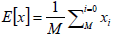
The CA CFAR processor updates threshold T by estimating the mean level in the window of M range cells as given by (Gandhi and Kassam, 1988),

(3)

This detector exhibits severe performance degradation in the presence of an interfering target in the reference window or in regions of abrupt change in the background clutter power (Gandhi and Kassam, 1988). Also, further false alarm rate degradation occurs if the extent of the clutter area is smaller than the window size (Gandhi and Kassam, 1988).

In the case of double target situation, the CA CFAR detector shows considerable deficiencies since any amplitude observed within the reference area simply is taken as clutter and no discrimination is possible between actual clutter returns and echoes of neighboring targets. The result is that one target may suppress the other or both targets may even remain undetected (Rohling, 1983).

OS CFAR

Another example is the OS CFAR detector proposed by Rohling, which has been considered to alleviate both of the above-cited problems. Furthermore, the OS CFAR processor may resolve multiple targets quite well, but it lacks of effectiveness in preventing excessive false alarms during clutter power transitions (Gandhi and Kassam, 1988).

In this algorithm the amplitude values taken from the reference window are first rank ordered according to increasing magnitude, i.e., x₁≤x₂≤...≤x_M. The central idea of OS CFAR procedure is to select one value x_k, where 1≤k≤M from the previous sequence, and to use it as an estimate for the average clutter power E[x] as observed in the reference window (Rohling, 1983).

The use of the ordered statistic in the context of CFAR processing does not define a single methodology but rather a series of different CFAR methods. For any given random variable x_k a distinct CFAR procedure is established. For practical application, only a few of the M possible values are of interest (Rohling, 1983). Though, the detection performance of the OS CFAR processor is independent of the location of the interfering targets in the reference window.

As a matter of fact, the OS CFAR detector, considering mean-level CFAR schemes, exhibits some loss of detection performance in homogeneous noise background compared with the CA processor, but its performance in a multiple target environment is clearly superior (Gandhi and Kassam, 1988).

C. CFAR threshold

When the clutter is modeled using a Weibull distribution, the detection threshold T can be obtained as a function of the clutter expectation E[x] and a scalar function of P_fa (Gálvez et al., 2011).

In the case of the CA CFAR, an estimate of E[x], μ, can be obtained by forming the mean value of samples taken from range cells leading, trailing or surrounding the CUT. Then, an estimate of threshold T, T', can be formed according to (Gálvez et al., 2011)

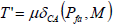(4)

where δ_CA(P_fa,M) is the CA CFAR threshold multiplier, a scalar function of P_fa and sample size M (Mahafza, 2000).

When working in homogeneous background, P_fa is maintained constant for the corresponding threshold multiplier. However, in situations of CB or MT, P_fa is no longer maintained and is drastically modified. By this reason, in presence of CB in the radar return, the threshold multiplier should be increased in order to maintain a constant P_fa. This problem occurs because the CA CFAR fails in the CB edges giving false detections.

On the other hand, the OS CFAR resolves closely spaced targets effectively for values of k (index associated to the CUT that represents the noise and clutter) different from the maximum (Gandhi and Kassam, 1988). The OS CFAR threshold is expressed as

(5)

where γ is the selected k-ranked cell to represent the noise and clutter level. The general expression for the P_fa, as a function of the actually used scale factor and the threshold multiplier in Weibull background is given by Levanon and Shor (1990)

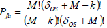(6)

Figure 2, shows the OS CFAR threshold multiplier δ_OS variation against the k sample for M=40, P_fa =1×10^-3 and P_fa =1×10^-5 for a Weibull background with parameters α=1 and Β=2. The curves were obtained by Monte Carlo simulation method. The results are very similar to those obtained by Eq. 6. The principal drawback of applying Eq. 6 is that only integer values of δ_OS should be used due to the factorial function, making it difficult to obtain results for intermediate values.

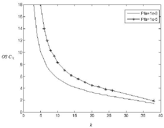
Figure 2: OS CFAR threshold multiplier δ_OS vs different k values for P_fa =1×10^-3 and P_fa =1×10^-5

III. NNCAOS CFAR

Additional motivations for developing a new CFAR method and a detailed description of the novel Neural Network Cell Average Order Statistic Constant False Alarm Rate(NNCAOS CFAR) detector are presented in the following.

A. Motivation for new CFAR methods

Excessive number of false alarms at clutter edges and degradation of the P_d in multiple target environments in the CA CFAR detector are the prime motivations for exploring other CFAR schemes that discriminate between interference and the primary targets (Gandhi and Kassam, 1988).

In the case of non homogeneous radar returns (with CB or MT), the CA CFAR P_fa is no longer constant. The samples corresponding to the CB and MT, are averaged in the CFAR window, resulting an overall threshold increase and false detections at clutter edges. On the other hand, OS CFAR detector is more robust than CA CFAR, especially when the k sample is high (near M). However, missing detection could occur in MT situations. The performance of this processor is highly dependent upon the values for k. Despite that OS CFAR detector exhibits some loss of detection performance in homogeneous noise background compared with CA CFAR, its performance in a multiple target environment is clearly superior (Gandhi and Kassam, 1988).

We take into account that the performance of the OS CFAR processor is highly dependent upon the values for k. For example, if a single extraneous target appears in the reference window of appreciable magnitude, it occupies the highest ranked cell with high probability. The estimate will almost always set the threshold based on the value of the interfering target. This results in an increase of the overall threshold and may lead to a target miss. If, on the other hand, k is chosen to be less than the maximum value, the OS CFAR processor will be influenced only slightly for up to M-k interfering targets (Gandhi and Kassam, 1988).

Of course, we are interested in both cases, i.e., regulating the false alarm at the clutter edges and minimizing target miss in the multiple target situations (Gandhi and Kassam, 1988). For this reason, different CFAR processors have been proposed to overcome the variety of situations that could be present within the radar return, i.e., CB, jamming, ice, multiple target, etc. (Gandhi and Kassam, 1988; Rohling, 1983; Haykin et al., 1991; Haykin and Deng, 1991; Smith and Varshney, 2000). If it were possible to have a priori knowledge of each situation, the most appropriate CFAR processor could be chosen for each case in order to achieve the best P_d while at the same time, to maintain intact the CFAR function that is to keep a constant false alarm rate.

Several authors have proposed different analytical methods to solve non homogeneous situations within the radar return (Smith and Varshney, 2000; Doyuran and Tanik, 2007). In this work, neural networks are proposed to take advantage of their efficiency (in terms of lower computation time than other schemes) considering real time processing (Gálvez et al., 2011). Using NN it is possible to make a classification to each radar return while working in real time. Haykin et al. (1991) and Haykin and Deng (1991) proposed a clutter classification methodology to distinguish between several mayor classes of radar returns including weather, birds and aircraft. Of particular interest is the use of a multilayer feedforward NN as the basis for classifying primary radar returns in, for example, aid traffic control environment applications (Haykin et al., 1991; Haykin and Deng, 1991).

CANN CFAR, presented in a former work, combines Maximum Likelihood (ML) for clutter parameter estimation, and NN for radar return homogeneity testing and clutter bank (transition points) and size estimation. It was demonstrated that this detector has better performance than conventional CFAR processors, especially when detecting targets located near clutter non homogeneities (Gálvez et al., 2011). An additional advantage of that technique is its efficiency when determining clutter transition points, bank size and threshold setting (Gálvez et al., 2011). On the other hand, it exhibits difficulties when discriminating multiple target, since it confuses multiple target situations with non homogeneities, diminishing in these cases the probability of detection considerability.

The NNCAOS CFAR is developed in this work with the purpose of improving the discussed difficulties. NN are used with the purpose of making a priori analysis to the radar return before an appropriate CFAR detector is applied. NNCAOS CFAR is a composed process, which takes advantage of NN as applied to CA CFAR and/or OS CFAR concepts.

B. NNCAOS CFAR description

Figure 3 depicts the NNCAOS CFAR block diagram. Like CANN CFAR, radar return enters to the Maximum Likelihood (ML) parameter estimation block where clutter parameters are estimated. We choose a relatively large number of samples (2M) at the end of the radar return for this estimation, assuming homogeneity. Then, we calculate the threshold multiplier for the CA CFAR process, δ_CA (P_fa,M), according to Gálvez et al. (2011), and use its value in the thresholding blocks.

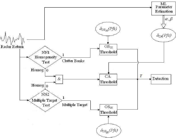
Figure 3: NNCAOS CFAR structure.

In the case of the OS CFAR processors, we obtain the threshold multiplier δ_OS (P_fa,M) from Fig. 2 for the corresponding kth sample and P_fa, assuming homogeneous clutter.

Two NN blocks, NN₁ and NN₂, analyze groups of M samples (M=40). NN₁ block searches for CB and NN₂ looks for MT. As a result, each sample is labeled as homogeneous, CB or MT. The algorithm selects a CA CFAR in the case of homogeneous radar return, an OS CFAR processor with a high kth sample (the OS₃₅. i.e., k=35 for the case of a CB, or the OS₂₀ for the case of a MT). Then, the most appropriate CFAR processor is applied to each sample in the CUT, and every CFAR processor obtains the threshold T, according to Eq. 4 and Eq. 5. Finally, the detection is carried out, a target is declared if the signal amplitude in the CUT is greater than the threshold.

We obtain thus, a robust system, which maintains a constant probability of false alarm P_fa even for non homogeneous returns while at the same time, it achieves a higher (or equal) probability of detection P_d than the classical systems in most of the cases.

IV. SIMULATION RESULTS

In this section, NNCAOS CFAR simulation results are shown in order to illustrate and discuss its performance.

A. NN training

NN training is performed by means of the backpropagation algorithm considering Weibull distributed radar returns. In the case of NN₁ homogeneity test block, a network composed by 40 inputs, 40 neurons in its hidden layer and only one output was trained for 20000 epochs by means of 6160 radar returns; 400 samples of homogeneous radar returns with diverse parameters (α=1; Β=2, 1.6, 1.4, 1.33), and 5760 samples with non homogeneous returns containing different size and parameter clutter banks situated at several positions (Gálvez et al., 2011).

The NN₂ multiple target test block, is also a neural network. This block with 40 inputs, 40 neurons in its hidden layer and only one output, was trained for 15060 epochs by means of 6655 homogeneous radar returns samples (without any target) and 6655 radar returns samples containing multiple targets situated at different positions within the CFAR window.

B. Performance Analysis

NNCAOS CFAR performance is compared to the CA, OS₂₀, the OS₃₅ and the CANN CFAR detectors. The results are illustrated in different figures. In these figures, we represent the NNCAOS CFAR with a right line, the CA CFAR with asterisks (*), the OS CFAR with a kth sample of 20 (OS₂₀) with a plus sign (+), the OS CFAR with a kth sample of 35 (OS₃₅) with a triangle (Δ) and the CANN CFAR with a circle (o). NNCAOS CFAR performance is compared to the other detectors for different representative radar return cases.

Case1: Homogeneous radar returns

P_d evaluation for the five detectors was performed using Monte Carlo simulations for 1000 Weibull radar returns containing 512 samples each.

Figure 4 depicts the detection performance for one of the four targets contained within the radar return. The other three targets exhibit very similar results. From the P_d curves we can conclude that in this case the performance detection is very similar for all CFAR detectors.

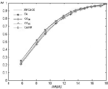
Figure 4: P_d for Case 1

Case 2: Radar returns containing a CB, and different isolated targets distributed along it, far away from the CB and any other target

Figure 5 shows the results of applying different CFAR processors over a radar return that contains a 20 sample CB. In the case of CA CFAR, the same as OS₂₀, have a low threshold over the CB producing thus false alarms in this sector. OS₃₅ CFAR presents the higher threshold levels, especially in the CB area. CANN CFAR misses the last target, but it has a good performance when avoiding the CB. In the case of NNCAOS CFAR, its threshold follows the CA CFAR in the homogeneous areas, while at the same time it is raised over the CB, pursuing OS₃₅ CFAR threshold. We also observe that OS₂₀ CFAR misses the last target and OS₃₅ presents a false alarm in the sample number 178. We can infer then, a better performance of NNCAOS CFAR that takes advantage of the benefits of applying a CA CFAR in the homogeneous areas, an OS₃₅ CFAR in the clutter areas and a OS₂₀ CFAR in the target areas, as evident from Fig. 5.

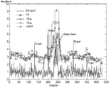
Figure 5: CFAR thresholds

P_d evaluation for the five processes was performed using Monte Carlo simulations for 1000 Weibull radar returns containing 512 samples each. Figure 6 shows the detection performance for one of the four targets contained within the radar return (the others exhibit very similar results). From P_d curves it is possible to conclude that NNCAOS CFAR has a similar performance to OS₃₅ CFAR, but superior to the CA, OS₂₀ and CANN CFAR when the same constant P_fa is maintained.

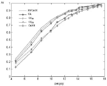
Figure 6: P_d vs SNR for one of the six targets contained within the radar return in Case 2.

We would expect that the OS₂₀ CFAR processor has a better detection performance, than the OS₃₅ CFAR due to its lower threshold dependent of the value of k. However, when the radar return contains CB, CA and OS₂₀ CFARs present an increment in P_fa especially in the clutter edges. For this reason, it was required to increment the threshold multipliers, 6.5 % for the CA CFAR, 15 % for the OS₂₀ CFAR and 5% for the CANN CFAR in order to maintain the same constant P_fa for the five processes (maintaining, in this manner, the same comparative rule). On the other hand, NNCAOS CFAR maintains a constant P_fa, independently of the radar return situation (homogeneous or not).

Case 3: Radar returns containing a CB and a group of four targets very near each other, but far away from the CB

P_d evaluation for the five CFAR detectors was performed using Monte Carlo simulations for 1000 Weibull radar returns containing 512 samples each.

Figure 7 shows the detection performance for this case. From P_d curves it is possible to conclude that the NNCAOS CFAR has the best performance for the four targets.

Figure 7: P_d vs SNR for Case 3

Considering that in this case the radar return contains CB, CA and OS₂₀ CFARs present an increment in P_fa especially in the clutter edges. For this reason, again, it was essential to increment the threshold multipliers, 6.5% for CA CFAR, 15% for OS₂₀ CFAR and 5% for CANN CFAR to hold the same constant P_fa for the four detectors. It is evident that CANN CFAR processor has the lowest detection performance because multiple targets are confused with non homogeities and avoided like a clutter bank, especially for the high SNR. On the other hand, NNCAOS CFAR maintains a constant P_fa, independently of the radar return situation (homogeneous or not).

Case 4: Radar returns containing a CB and a group of targets very near each other and the CB

P_d evaluation for the five CFAR processes was performed using Monte Carlo simulations for 1000 Weibull radar returns containing 512 samples each.

Figure 8 shows the detection performance for this case. From P_d curves it is possible to conclude that NNCAOS CFAR has the best performance for the first and the last targets. In the case of the targets that are very near the clutter bank, CANN CFAR has a considerable better performance than the other detectors, especially for low SNR. This is due to its especial ability to detect targets located near clutter non homogeneities (Gálvez et al., 2011). In the case of the last target, the performance of NNCAOS CFAR and OS₃₅ CFAR are at higher than the performance of the other detectors. From Fig. 8 it can be noticed that NNCAOS CFAR has a high detection performance for all the cases, while the other four CFAR detectors performance fluctuate according to the target position. Considering that in this case the radar return contains CB, CA and OS₂₀ CFAR present an increment in the false alarm rate especially in the clutter edges. For this reason, it was essential to increment the threshold multipliers, 5.6 % for the CA CFAR, 12 % for the OS₂₀ CFAR and 5% for the CANN CFAR to hold the same constant P_fa for the four processes. On the other hand, NNCAOS CFAR maintains a constant P_fa, independently of the radar return situation (homogeneous or not).

Figure 8: P_d vs SNR for Case 4

V. CONCLUSIONS

We have studied four possible environment cases to investigate NNCAOS CFAR performance and compare it to other classical processes, CA, OS CFAR and a previously proposed NN based CANN CFAR detector (Gálvez et al., 2011). From Case 1, it is possible to conclude that NNCAOS CFAR has a similar performance than CA and OS CFAR detector when working with homogeneous radar returns. In Case 2 we found that the performance of NNCAOS CFAR is very similar to that of OS₃₅ CFAR and superior to that of CA, OS₂₀ and CANN CFAR (for equal P_fa) when the radar return contains a CB, and different isolated targets. On the other hand, NNCAOS CFAR maintains a constant P_fa, independently of the radar return situation (homogeneous or not). In Cases 3 and 4 NNCAOS CFAR performance was studied when the radar return contains a CB and a group of four targets very near each other, far away or near the CB. We can conclude that NNCAOS CFAR has the best performance for some of the targets while at the same time it maintains a constant P_fa, independently of the radar return situation (homogeneous or non homogeneous). In summary, the great advantage of NNCAOS CFAR detector is that it presents a higher Pd performance than CA, OS and CANN CFAR schemes for most of the cases while at the same time it maintains a constant P_fa even for non homogeneous radar returns. This makes it a robust detector, as opposed to the CA, OS or CANN CFAR, that increment their false alarm rate under non homogeneities.

Notas
¹ Optimality can be shown when the reference cells contain independent and identically distributed (IID) observations governed by an exponential distribution.
² The Beaufort scale is used as a measure of the wave height, classifying the sea in 10 levels with wave height of 0 feet to 45 feet.

REFERENCES
1. Doyuran, U.E. and Y. Tanik, "Detection in range-heterogeneous weibull clutter," IEEE Radar Conference, 343-347 (2007).
2. Gandhi, P.P. and S.A. Kassam, "Analysis of CFAR processors in nonhomogeneous background," IEEE Transactions on Aerospace and Electronic Systems, 24, 427-445 (1988).
3. Gálvez, N.B., J.E. Cousseau, J.L. Pasciaroni and O.E. Agamennoni, "Efficient non homogeneous CFAR processing," Latin American Applied Research, 41, 1-9 (2011).
4. Haykin, S. and C. Deng, "Classification of radar clutter using neural networks," IEEE Transactions on Neural Networks, 2, 589-600 (1991).
5. Haykin, S., S. Stehwien, C. Deng, P. Weber and R. Mann, "Classification of radar clutter in an air traffic control environment," Proceedings of the IEEE, 79, 742-772 (1991).
6. Levanon, N. and M. Shor, "Order statistics cfar for weibull background," IEEE Proceedings, 3, 157-162 (1990).
7. López Estrada, S., R. Cumplido Parra, and C. Torres Huitzil, "A hybrid approach for target detection using CFAR algorithm and image processing," IEEE, Proceedings of the Fifth Mexican International Conference in Computer Science (2004).
8. Mahafza, B., Radar Systems Analysis and Design Using Matlab, Chapman and Hall, CRC, 172-175 (2000).
9. Minkler, G. and J. Minkler, The Principles of Automatic Radar Detection In Clutter. CFAR, Magellan Book Company, Baltimore, MD. Palm Bay (1990).
10. Rifkin, R., "Analysis of CFAR performance in weibull clutter," IEEE Transactions on Aerospace and Electronic Systems, 30, 315-328 (1994).
11. Rohling, H., "Radar CFAR thresholing in clutter and multiple target situations," IEEE Transactions on Aerospace and Electronic Systems, 19, 608-621 (1983).
12. Smith, M.E. and P. Varshney, "Intelligent CFARB processor based on data variability," IEEE Transactions on Aerospace and Electronic Systems, 36, 837-847 (2000).

Received: August 19 2011
Accepted: January 5, 2012
Recommended by subject editor: José Guivant