Harmonic disturbance rejection control for magnetic field compensation applications

G. O. Forte and E. Anoardo

^† LaRTE, Grupo de Resonancia Magnética Nuclear, Facultad de Matemática Astronomía y Física, Universidad Nacional de Córdoba and IFEG (CONICET), Argentina. forte@famaf.unc.edu.ar, anoardo@famaf.unc.edu.ar

Abstract— A simple control strategy was studied for harmonic disturbance rejection in magnetic field compensation systems for lowfield magnetic resonance techniques. The strategy is based on the simultaneous action of a conventional PID and a selective harmoniccompensation controller. The system consists of a set of compensating coils fed by independent current sources driven by a digital controller. A series of hall magnetic sensors close the control loop. Despite its simplicity, it is shown that the performance of the dual controller improves within the frequency range where the waterbed effect becomes dominant, by selectively enhancing the rejection of the harmonic component. The proposed solution is particularly useful for selective harmonic rejection of slowly varying frequency and amplitude dependent harmonic perturbations. An extension to multiple-harmonic components perturbations is possible.

Keywords— Automatic Frequency Control; Waterbed Effect; Harmonic Rejection; Periodic Control.

I. INTRODUCTION

Field-cycling nuclear magnetic resonance (NMR) techniques require magnetic field compensation in order to run experiments at very low or zero-field conditions (Anoardo and Ferrante, 2003). In NMR relaxometry applications, it is desirable to extend the operative magnetic field range of the hardware in order to scan relaxation parameters up to very weak magnetic fields (Kimmich and Anoardo, 2004). A magnetic field compensator is also atractive for Zero-field NMR spectroscopy and double resonance nuclear quadrupole spectroscopy (NQR) as well. More recently, fieldcycling magnetic resonance imaging (MRI) has been performing as a new paradigm of potential massive use in medical diagnosis (Lurie et al., 1998; Matter et al., 2006). For all of these, a quality compensation of the magnetic field not only demands for cancellation of time-independent components, but also for timedependent and harmonic contributions arising from the environment.

The problem is more general however. There are many applications where the attenuation or cancelation of periodic disturbances are necessary. Active shielding (Kuriki et al., 2002; Platzek et al., 1999; Sergeant et al., 2003; Sergeant et al., 2007; ter Brake et al., 1993) and active noise cancellation (Kuo and Morgan, 1999; Nelson and Elliot, 1992) are examples. The problem of rejecting periodic disturbances with uncertain frequency is common in mechanical and electronic systems. Different solutions were considered, as for example, adaptive algorithms to estimate the frequency and the amplitude of the disturbance in combination with a phase-locked loop (Bodson and Douglas, 1997) or, internal model (IM)-based adaptive algorithms (Brown and Qing Zhang, 2004).

In most cases, the solution is based on controllers operating in the time domain. In the case of a noise perturbation composed of several frequency components, those within the bandwidth of the controller will be attenuated, while those occurring at higher frequencies will be amplified; phenomena called "waterbed effect" (Skogestad and Postlethwaite, 2005). If these last components can be selectively mitigated by other means, it would be possible to extend the effective dynamic range of the controller, while keeping the required quality of attenuation within the bandwidth of the controller. This strategy cannot be implemented with a conventional feedbacked controller working in the time domain. Feedforward controllers are not subjected to the waterbed effect, but can only be used for a detailed plant estimation and a harmonic spectrum constant in time (Akogyeram and Longman, 2001). In this work, a controller that combines the action of both, time and frequency domains, fixing the waterbed effect problem is presented. The used frequency domain algorithm is related to the more sophisticated gradient algorithms (Nelson and Elliot, 1992), and also to higher harmonic control (HHC) or Multicyclic Control (Johnson, 1982; Patt et al., 2005).

The simplification in the proposed method relays in the use of the Fast Fourier Transform (FFT) to extract the information from the measured output signal, necessary to close the control loop using a simple PI controller. This is an important characteristic of the algorithm since, in the context of the present problem, it is not possible to measure the perturbation alone as it is frequently done in active noise cancellation.

In this manuscript we deal with a magnetic field active shielding system designed for Fast Field Cycling (FFC) Nuclear Magnetic Resonance (NMR) experiments. The experimental situation has already been described in an earlier publication (Forte et al., 2010).

II. CONTROL STRATEGY

Non-periodic disturbances are canceled with a conventional PID controller (C1) working in the time domain. A second PI controller (C2) working in the frequency domain is added to deal with harmonic perturbations (Fig. 1). Controller in the time or frequency domain refers to how is it expressed its input signal (Palani, 2010). While C1 works with the signal as it is measured by the magnetic field sensor, C2 works with its Fourier Transform.

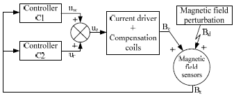
Figure 1: Description of the system

If a harmonic component occurs at a frequency where the waterbed effect manifests for C1, the action of C2 will compensate the effect thus extending the dynamic range of the combined system.

All magnetic fields are time-dependent. For simplicity, it is not included the time dependence (t) of the different magnetic field variables explicitly in the text. The relevant signals affecting the system of Fig. 1 are:

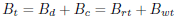(1)

where B_t is the total magnetic field sensed, B_d represent all the disturbances, B_c is the compensating magnetic field, B_rt is the f_r frequency component of the total magnetic field and B_wt includes all frequency components of B_t different from f_r.

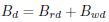(2)

where B_rd is the armonic disturbance that will be cancelled by C2 and B_wd represents all other disturbances that will be cancelled by C1.

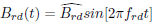(3)

where is the amplitude of B_rd(t) and f_rd is the B_rd frequency of B_rd(t).

(4)

where B_rc is the compensation signal generated by C2 and B_wc is the compensation signal generated by C1.

(5)

where is the amplitude of B_rc(t), f_rc is the frequency of B_rc(t)and θ_rc(t) is the phase of B_rc(t)with respect to B_rd(t).

For any controller working in harmonic noise mitigation, the solution will be equivalent to the addition of an antiphase signal, with same frequency and amplitude than that of the perturbation. If the parameters ( and f_rd) of the harmonic perturbation (Eq. 3) are well known, itispossibletoeliminate B_rd if we do:

	(6)
	(7)
	(8)

where K_ri is a design parameter, T is the control loop period of C2 and B_rn is the normalized amplitude of B_rt defined as .

If Eqs. 6 and 7 hold, it is possible to find a value of K_ri (Eq. 8) that satisfies θ_rc(t) → π when t → ∞.As it is assumed constant (or slowly varying) frequency and amplitude characteristics for the harmonic component of the perturbation B_rd, both and f_rd can be approximated through a high-resolution FFT before starting the active cancellation process. Once the controllers are fully active, B_rt is cyclically calculated trough a fast FFT performed on the samples acquired during the C2 loop period (T).

	(9)
	(10)
	(11)

where: k is the control iteration index.

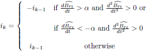α is a design parameter used to introduce a hysteresis in the swith condition of i_k. For the first iteration (k =1) i_k is initilized with 1.

In Eq. 11, the sign of the integral argument is changed every time B_rt passes throught a minimum. In this way, it is possible to keep both signals (B_rd and B_rc) near antiphase, although their magnitude were different. In steady state, the system behaves as an on-off controller, keeping B_rt oscillating around their minimum value (amplitude modulation -AM -with a small depth index). This behavior seems to be a common feature of this kind of controllers (see for instance Sergeant et al., 2007). The amplitude of the oscillation depends on the time interval between the moment at which B_rt reaches the minimum, and the change in the sign of the C2 integral argument (Eq. 11). Ideally, if this time interval is reduced to zero, the amplitude of the oscillation cancels (there is no modulation). However, for robustness, it is mandatory to admit a certain hysteresis (like in every on-off controller) by setting α > 0.

It is desired that the total magnetic field at f_r frequency never becames larger than the disturbance at the same frequency, that is:

(12)

This condition can be expressed in therms of the phase angle:

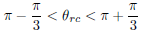(13)

Which implies that it must be satisfied that:

(14)

As B_rn is normalized, its maximum possible value is 2 (when B_rc and B_rd are in phase). Then,

(15)

Now, if the disturbance frequency suddenly change, making while the amplitude does not suffer any change, the envelope of the sum of B_rc + B_rd will be:

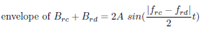(16)

where .

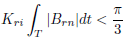
Using Eq. 16, to preserve inequality 12, it must be satisfy that:

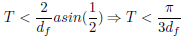(17)

.

Since the dynamics of the plant is intrinsically driven by the control algorithm of C2, the command signal u_c applied to the plant will just depend on the gain K_p of the plant transfer function:

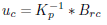(18)

where K_p is the gain of the plant transfer function.

Controllers C1 and C2, do not affect their performance each other. C1 can only modify the magnitude of the disturbance view by C2, but in steady way over time. In addition, C1 views the magnetic field generated by C2 as any other perturbation.

III. SIMULATED ALGORITHM PERFORMANCE TESTS

The algorithm was applied to a controller aimed for a magnetic field active shielding (Forte et al., 2010). The controlled variable B_c(t) is the mean magnetic field along one axis direction. The actuator consists of a set of coils generating a homogeneous magnetic field along the same axis of B_r(t). The current flowing through these coils are handled by the combined action of controllers C1 and C2. The plant is modeled by a second order transfer function with delay:

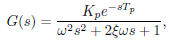(19)

where G(s) is the transfer function in the Laplace domain (s), T_p is the time delay [s], ξ is the damping factor and ω is the natural frequency [r/s].

The transfer function parameters values are: K_p = 25.54, T_p = 510e-5, ξ = 0.647 and ω = 1.4e3 (Forte et al., 2010).

Simulations were carried out using the Simulink toolbox of MatLab. A general block-scheme of the system can be observed at Fig. 2. The plant has been modeled with a linear transfer function of second order, including delay and a saturation block representing the largest current output allowed by the hardware (Fig. 3a). As an example, it can be considered here the case where the system has to deal with a perturbation composed of two definite frequency components and an offset (Fig. 3b).

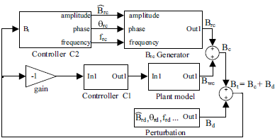
Figure 2: Simulation model: general diagram.

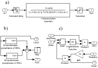
Figure 3: Details inside blocks of Fig. 2: a) Plant model. b) Perturbation (with two frequency harmonic components and offset) and c) B_rc generator.

C1 attenuates constant disturbances and one of the harmonics (with its frequency defined within the bandwidth of the controller). A compensating signal was added to cancel the second harmonic, with frequency defined within the range where the waterbed effect dominates the response of the C1 controller. This signal is generated by the subsystem shown in Fig. 3c and it is managed by the specifically designed controller C2.

The input signal to the C1 controller is the error e defined as follows:

(20)

where c is the controlled variable and r is the reference signal.

The purpose of the control is to cancel the magnetic field, that is, e(s)= −c(s). The PID controller equation (Ziegler and Nichols, 1942) is:

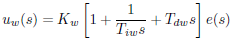(21)

where u_w(s) is the controller output and the plant input and K_w, T_iw and T_dw are the parameters of the controller.

The controller was tuned following the Sung method (Sung et al., 1998) (K_w = 13.6e-3, T_iw = 2.7 and T_dw = 1.5e-3). Simulations were done by discretization (Ogata, 1987).

When the frequency domain controller C2 is turned on, a FFT with a large number of samples is performed to determine the amplitude and frequency of the perturbation (B_rd and f_rd). During this step, both controllers are inoperative. Once the system is fully working, a faster FFT (few samples) is cyclic performed to close the loop of the phase-tracking procedure. The subsystem that tracks the phase, integrates all the time the amplitude component of the resulting magnetic field B_rc(t) + B_rd(t) at f_rc frequency. This feedback signal is normalized dividing it by , in order to keep the loop gain independent of the perturbation intensity.

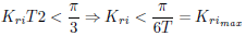
Parameters of controller C2 were set as follow: Sample frequency f_s =1KHz, control loop period T = 64ms, K_ri = 5 < π / (6 ∗ T). So, the largest possible change of the disturbance frequency during T is: .

The most important block of this controller is that checking the sign of the integral argument, used to define the sign of the phase step of θc(t). The decision of switching from phase increment to phase decrement (or vice versa) is taken in the moment at which the perturbation intensity crosses a minimum (see Fig. 4). A moving average filter is applied before and after calculating the derivatives. A J-K flip-flop managed by the sign of the previously calculated derivative detects the condition of passing through a minimum. At the end of this block, the output is multiplied by the absolute value of the derivative, only when B_rt is decreasing in time.

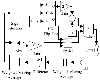
Figure 4: Details of the block involved in the minimum intensity condition detection for the phase-tracking algorithm.

Initially, C1 was tested with two frequency components (20Hz and 80Hz), one within the bandwidth of the controller, and the other in the range where the PID amplifies. Frequencies beyond the limit imposed by the sample rate will be rejected by the antialiasing filter and will not be affected by the system (Oppenheim et al., 1983). In turn, a step was added at t = 3.5s. As expected, the low-frequency component is attenuated while the other is amplified. The C1 controller behaves satisfactorily with the step perturbation, which drives it to zero immediately. The same perturbation was later applied to C2. Since the algorithm was designed to cancel only one frequency component (the highest), C2 attenuates that component without affecting the other. However, the step is not affected by this controller.

Figure 5 shows the simulated result when both C1 and C2 are working simultaneously. At t = 2.5s C2 starts attenuating the perturbation using the information recovered until that time. C1 is turned on at t = 3s. Two small lateral bands arise around the frequency component of 80Hz as a consequence of the AM modulation effect of the C2 controller. The total disturbance spectral energy is conveniently reduced when both controllers are working.

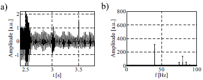
Figure 5: a) Total magnetic field when both controllers are active. At time t=3.5s a step perturbation is introduced. b) Spectrum of the magnetic field after the step perturbation have been added.

IV. EXPERIMENTAL

Experiments were carried out using the platform already described in Forte et al., 2010. A new dedicated hardware executes the control tasks that were previously based on PC environment. The system is based on a TMX320F28335 digital signal controller (DSC). The magnetic field feedback information is read from the hall sensors using two MAX1316 analogue to digital converters (ADC), providing 10 input channels. The controller also has 8 analogue outputs provided by two DAC8544 digital to analogue converters (DAC), used to manage the currents flowing through the compensating coils. Data are moved between ADCs and the DSC by direct memory access (DMA) thus optimizing the system speed. The control loop sample time is governed by an internal timer which reduces the hitter to the minimum. This issue critically affects the performance of the controller, being however this a minor problem at the present stage of concept testing.

As a first experiment, the frequency response of C1 was characterized. The waterbed effect starts to manifest at a frequency of about 10Hz. In contrast to C1, controller C2 does not have a region where disturbances are amplified, but if a step is applied, this controller has no effect (Fig. 6a). The two controllers have been lump together resulting in a system with good frequency characteristics and capability of step compensation (Fig. 6b). Experiments of Fig. 6 were done with a perturbation having its frequency within the bandwidth of C1. Figure 7 shows that the negative effect of C1 at a frequency where the waterbed effect dominates, can be practically eliminated by the action of C2, when both controllers are working.

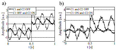
Figure 6: a) The controller C2 can attenuate a harmonicu perturbation but has no effect if a step is introduced. b) The combination of both controllers (C1 and C2) results in a system that con diminishes both kinds of perturbations.

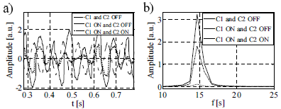
Figure 7: System behavior for a perturbation of frequency where C1 acts as an amplifier. a) Time domain signals. b) Spectral representation.

V. DISCUSSION

A deficiency of the proposed solution is related to the phase-tracking algorithm. A hysteresis is introduced from the determination of the sign of the phase steps (increments or decrements) which is based on the calculation of derivatives. As this operation is highly sensibly to noise, the controller changes the sign of the feedback signal before B_rt passed through its minimum value. This situation would produce a momentarily loss of control, resulting in an undesirable peak in B_rt (of magnitude ). The added hysteresis demands checking that dB_rt/dt remains positive for a while after crossing the minimum.

The amplitude and frequency of the compensating signal differ from the real disturbance due to unavoidable errors of the FFT. The controller must be constantly tracking the phase of B_rd(t) to cancel the harmonic perturbation, thus imposing a frequency limit for the algorithm loop. Moreover, every control loop, the FFT of B_t(t) is performed to measure the feedback signal. This FFT should have the minimum quantity of samples needed to characterize B_rt, also affecting the frequency response of the controller. Therefore, the algorithms used to measure the frequency and amplitude of the perturbation and the phase-tracking procedure, are critically affecting the dynamic range of thesystem. This drawback couldbeovercameby sensing the perturbation outside the exclusion volume and using a feedborward controller. However, in our application, the surroundings of the exclusion volume are affected by the time dependent disperse field of the main magnet of the relaxometer.

Unlike other control strategies, like repetitive control (Hara et al., 1985) or iterative learning control (Arimoto et al., 1986), the simple method proposed in this work can selectively reject harmonic perturbations. This is an important issue when, at the output of the system, the perturbation contains harmonic components that should remain unaffected. Existing control strategies for the rejection of harmonic components are based on the estimation of the main component (see for example Bodson et al., 2001). In this work, every control cycle the systems seeks perturbation information, thus avoiding the risk that the estimator does not converge. If for any circumstance, the controller looses the control of the antiphase signal, the system recovers itself after a transient time where the perturbation can be amplified at most by a factor of two.

VI. CONCLUSIONS

It was shown that the waterbed effect associated to controlled signals in the time domain can be circumvented with the addition of a conventional PI controller working in the frequency domain. In this way, thedynamic rangeand theperformance of thecombined controller can be improved. A deeper mathematical analysis is needed to explore the limits of operation, particularly analyzing other alternatives to the FFT and the phase-tracking algorithms. The present scheme can be adapted for the selective rejection of two or more harmonic components, particularly in the case of steady conditions. Experimental results depicted in Fig. 7 clearly shows that the practical implementation of the proposed solution, although involving very simple control concepts, can be extremely efficient.

ACKNOWLEDGEMENTS
The Authors acknowledge the financial support from MINCYT Córdoba, SECyT-UNC and CONICET. We thank to B. Reyes, W. Salinas and F. Barra for the collaboration in the implementation of the new hardware.

REFERENCES
1. Akogyeram, R. A. and R. W. Longman, "On the choice of the method to cancel 60Hz disturbances in the beam position and energy," Proceedings of the 2001 particle acelerador conference, Chicago, EEUU, 1270-1272 (2001).
2. Anoardo, E. and G. Ferrante, "Magnetic Field Compensation for Field-Cycling NMR Relaxometry in the ULF Band," Appl. Magn. Reson., 24 , 85-96 (2003).
3. Arimoto, S., S. Kawamura and F. Miyazaki, "Convergence, stability and robustness of learning control schemes for robot manipulators," Proceedings of the International Symposium on Robot Manipulators on Recent trends in robotics: modeling, control and education, 307-316 (1986).
4. Bodson, M. and S. C. Douglas, "Adaptive algorithms for the rejection of sinusiodal disturbances with unknown frequency," Automatica, 33, 2213-2221 (1997).
5. Bodson, M., J. S. Jensen and S.C. Douglas, "Active noise control for periodic disturbances," IEEE Transactions on control systems technology, 9, 200-205 (2001).
6. ter Brake, R. Huonker and H. Rogalla, "New results in active noise compensation for magnetically shilded rooms," Meas. Sci. Technol., 4, 1370-1375 (1993).
7. Brown, L. J. and Qing Zhang, "Periodic disturbance cancellation with uncertain frequency," Automatica, 40, 631-637 (2004).
8. Forte, G. O., G. Farrher, L. R. Canali and E. Anoardo, "Automatic Shielding-Shimming Magnetic Field Compensator for Excluded Volume applications," IEEE Transactions on control systems technology, 18, 976-983 (2010).
9. Hara, S., T. Omata and M. Nakano, "Synthesis of repetitive control systems and its application," Proceedings of the 24th conference on decision and control, 1387-1392 (1985).
10. Johnson, W., Self-tuning regulators for multicyclic control of helicopter vibration, National Aeronautics and Space Administration, Scientific and Technical Information Branch, Washington, D.C (1982).
11. Kimmich, R. and E. Anoardo, "Field-cycling NMR Relaxometry," Progress in nuclear magnetic resonance spectroscopy, 44, 257-320 (2004).
12. Kuo, S. M. and D. R. Morgan, "Active noise control: a tutorial review," Proc. IEEE, 87, 943-973 (1999).
13. Kuriki, S., A. Hayashi, T. Washio and M. Fujita, "Active compensation in combination with weak passive shielding for magnetocardiographic measurements," Rev. Sci. Instrum., 73, 440-445 (2002).
14. Lurie, D. J., M. A. Foster, D. Yeung and J. M. S Hutchinson, "Design, construction and use of a large-sample field-cycled PEDRI imager," Physics in Medicine and Biology, 43, 1877-1886 (1998).
15. Matter, N. I., G. C. Scott, T. Grafendorfer, A. Macovski and S. M. Conolly, "Rapid polarizing field cycling in magnetic resonance imaging," IEEE Transactions on Medical Imaging, 25, 84-93 (2006).
16. Nelson, P. A. and S. J. Elliot, Active control of sound, Academic Press, San Diego (1992).
17. Ogata, K., Discrete-Time Control Systems, Prentice Hall, Upper Saddle River, New Jersey (1987).
18. Oppenheim, A. V., A. S. Willsky and I. T. Young., Signals and systems, Prentice Hall, Englewood. Cliffs, New Jersey (1983).
19. Palani, S., Control Systems Engineering, Tata Mc-Graw Hill, New Delhi (2010).
20. Patt, D., L. Liu, J. Chandrasekar, D. S. Bernstein and P. P. Friedmann, "Higher-Harmonic-Control Algorithm for Helicopter Vibration Reduction Revisited," Journal of guidance, control, and dynamics, 28, 918-930 (2005).
21. Platzek, D., H. Nowak, F. Giessler, J. Röther and M. Eiselt, "Active shielding to reduce low frequency disturbances in direct current near biomagnetic measurements," Rev. S. Instrum., 70, 2465-24709 (1999).
22. Sergeant, P., L. Dupré, M. De Wulf and J. Melkebeek, "Optimizing Active and Passive Magnetic Shields in Induction Heating by a Genetic Algorithm," IEEE Trans. Magn., 39, 3486-3496 (2003).
23. Sergeant, P., A. Van Den Bossche and L. Dupré, "Hardware control of an active magnetic shield," IET Sci. Meas. Technol., 1, 152-159 (2007).
24. Skogestad, S. and I. Postlethwaite, Multivariable feedback control. Analysis and Design, John Wiley and Sons, Ltd., Chippenham, Wiltshire (2005).
25. Sung, S. W., I. B. Lee and J. Lee, "New process identification method for automatic design of PID controllers," Automatica, 24, 513-520 (1998).
26. Ziegler, J. G. and N. B. Nichols, "Optimum settings for automation controllers," Transactions of the ASME, 64, 759-768 (1942).

Received: June 28, 2011.
Accepted: May 4, 2012.
Recommended by Subject Editor José Guivant.