A new inverse kinematic algorithm for discretely actuated hyper-redundant manipulators

A. Motahari^†, H. Zohoor^‡ and M.h. Korayem^§

^† PhD student, Department of Mechanical and Aerospace Engineering, Science and Research Branch, Islamic Azad University, Tehran, Iran, POB: 14155-4933, Corresponding author. a.motahari@srbiau.ac.ir
^‡ Professor, Center of Excellence in Design, Robotics and Automation, Sharif University of Technology; Fellow, The Academy of Sciences of IR Iran, zohoor@sharif.edu
^§ Professor, Center of Excellence in Experimental Solid Mechanics and Dynamics, Iran University of Science and Technology, hkorayem@iust.ac.ir

Abstract— The term discretely actuated hyper-redundant manipulator is applied to a kind of manipulators which consists of serially connected modules. Such modules are composed of discretely actuated joints having finite stable states. Since the previous studies have rarely offered satisfactory results regarding the problem of inverse kinematics of discretely actuated hyper-redundant manipulators, the present study is attempting to develop and investigate an effective algorithm to solve this problem. To achieve this, the current research intends to solve the problem of 2D and 3D inverse kinematics of manipulators with many modules, by considering both position and orientation of end frame in real-time with fairly high accuracy. The main ideas of the proposed method are: using mean workspace, breadth-first search with two non-adjacent modules in each step and improving the results by iterating the process. The effectiveness of the presented method is verified through different numerical analyses for various case studies.

Keywords— Binary Manipulators; Discrete actuation; Hyper-redundant Manipulators; Inverse Kinematics.

I. INTRODUCTION

A hyper-redundant manipulator can be produced by cascading serial and/or parallel manipulators -as modules- on top of one another with a fixed base. This way, the manipulator is like a serial robot in a macroscopic view (Ebert-Uphoff and Chirikjian, 1996). In the present article, whenever we use the term 'hyper-redundant manipulator' we are, in fact, referring to the manipulator type that was introduced above. The serial connection of modules in these manipulators causes their workspace to be large. Furthermore, their large degree of freedom results in high dexterity and the ability to avoid obstacles by their snake-like motions. However, it also causes complexity in control. To overcome this limitation, the discrete actuators are proposed instead of traditional continuous ones. A discrete actuator has only a few stable states. For example, a binary prismatic actuator has only two possible states, either fully extended or fully retracted. A Discretely Actuated Hyper-redundant Manipulator (DAHM) is a hyper-redundant manipulator with all of its active joints actuated discretely. The joint level control in DAHMs is very simple because of the simple mechanism of the discrete actuators. So the control does not require feedback sensors (Sujan and Dubowsky, 2004). It makes DAHMs cheaper and lighter than the hyper-redundant manipulators which contain continuous actuators. High task repeatability and high reliability are the other advantages of DAHMs developed by simplicity of their joint level control. In fact the application of discrete actuators is not restricted to hyper-redundant manipulators. For some examples readers are referred to Proulx and Plante (2011), Chen et al. (2011) and Petit et al. (2010).

Since the actuators of a DAHM have only a few stable states, possible configurations of a DAHM are limited to several states. The number of possible configurations grows exponentially by increasing the number of modules. For example, if each module contains three binary actuators, then the number of configurations of each module will be eight. Now if five of these modules are connected serially, then the constructed manipulator will have 8⁵=32,768 configurations. The position of the end frame related to each configuration specifies a point of the manipulator workspace, so the workspace of a DAHM is a cloud of discrete points.

One of the most important issues in kinematic analysis of DAHMs is the inverse kinematic problem. Since the solution of forward kinematics of these manipulators is clarified, the first idea for solving the inverse kinematic problem that comes to mind is to solve forward kinematic of all possible configurations offline, saving all positions of the end frame of the manipulator with their corresponding configurations, and using them online. But due to the exponential growth of the number of the possible configurations, this method is not feasible for the manipulators which contain a high number of modules, both in terms of the solution time and the required memory.

On the other hand, a DAHM will be practical only if the number of modules is high. Thus, finding an efficient method for solving the inverse kinematic problem of DAHMs is essential.

Until now, many efforts have been made to solve this problem. Chirikjian and Lees (1995) approximate macroscopic feature of the manipulator by a special curve which they named as "backbone curve". They solved the inverse kinematic problem in two steps; calculating the parameters of the curve was done at first and then the DAHM was adhered to the curve. Nevertheless, it was usually impossible to fit the DAHM on the curve precisely, because the active joints only accepted the discrete amounts. This caused large position errors in their solution method.

Ebert-Uphoff and Chirikjian (1995, 1996, 1998) defined and evaluated the workspace density of DAHMs and used it to solve the inverse kinematic problem. In their method, the workspace was divided into some pixels and the workspace density of each pixel was evaluated and memorized. For more accuracy it was necessary to use smaller pixels. This made the number of the pixels very huge, especially in 3D cases and therefore the offline solution time and required memory would be very high. Suthakorn and Chirikjian (2001) proposed a method which can evaluate the mean position of the workspace of the DAHMs very fast. They used the mean position to solve the inverse kinematic problem. Their method was very fast and the amount of the data that was needed to be stored was small, but it had large errors.

Some investigators (Sujan and Dubowsky, 2004; Scofano, 2006) used a genetic search algorithm to solve the inverse kinematic problem of the manipulators with a large number of binary actuators. In their method, it was necessary to increase the size of the search space explored by the genetic algorithm to achieve reasonable accuracy. This increases the solution time to several seconds.

In this paper a new inverse kinematics algorithm is proposed, which has all of these benefits together: 1) it solves DAHM inverse kinematic problem with many modules over a period of time less than a second; 2) the results are fairly accurate; 3) the solutions can be improved by iterations of the algorithm; 4) it can consider both position and orientation in solution; 5) it is suitable for 2D and 3D problems; 6) it can be used for manipulators with dissimilar modules.

Suthakorn's method (Suthakorn and Chirikjian, 2001) is modified using two heuristic ideas to decrease the errors. The first idea is determining the configuration of two non-adjacent modules in each step of breadth-first search method which improves the accuracy. The second idea is iterating the algorithm, which makes the results better. The effectiveness of the proposed method for solving the inverse kinematic problem of DAHMs is verified by 2D and 3D case studies and the results are compared with the results of Suthakorn's method and Genetic Algorithm (GA) method.

The remainder of this article is organized as follows. Section 2 introduces Suthakorn's method, the two ideas used in this paper and GA method. Finally the error is defined. Section 3 expresses two algorithms for solving the inverse kinematic problem based on the two ideas. Section 4 introduces two 2D and a 3D manipulator and their numerical results. Section 5 is the conclusion.

II. FUNDAMENTALS

A. Introducing DAHM inverse kinematic problem

To clarify the issue, a 2D manipulator, which its modules include a link that sticks to the previous module with a revolute joint, is considered. This module is called 'R-link' here. As shown in Fig. 1, each joint can be actuated in one of the two angles of -20 or 20 degrees. Configuration 1112 of a four-module manipulator is illustrated in Fig. 2. In this configuration code, number 1 denotes the -20 degrees actuation, and number 2 refers to the 20 degrees actuation. The i^th digit of configuration code illustrates the configuration of i^th module which starts from the base.

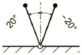
Fig. 1: Configurations of a binary R-link module; the angles of -20 and 20 degrees are related to configurations 1 and 2, respectively.

Fig. 2: Configuration 1112

In DAHM inverse kinematics problem, we are looking for a configuration as an answer, where the corresponding end frame is as close as possible to a prescribed frame, named 'target frame' or in short 'target'. This requires a definition for distance between two frames including both location and orientation differences. In this paper we use Park's definition (Park, 1995). These are described in Appendix A. Now, if the target frame is obtained by solving direct kinematics for a prescribed configuration, then there will be an exact solution for inverse kinematic problem, and the distance between the end frame and the target frame can be considered as an error.

B. Suthakorn's method

As mentioned earlier, with some modifications, Suthakorn's method (Suthakorn and Chirikjian, 2001) is used to solve the inverse kinematic problem in this paper. First, Suthakorn's method is introduced briefly. In Suthakorn's method the configuration of one module is selected among all its configurations at each step of the solution. This selection starts from the base module and is continued to the end module. This selection is based on probabilities. It means that the selection criterion is the probability of reaching the target frame. This probability is more when the density of the manipulator workspace at the neighborhood of target frame is high. In Suthakorn's method it is assumed that the densest position of the workspace is its mean position, and the workspace density decreases with the distance of the mean position. Therefore, if the distance between the end frame and the mean frame decreases, then the related workspace density is increased. Calculating the mean frame of the manipulators can be done easily by the method proposed by Suthakorn and Chirikjian (2001). This method is described briefly in Appendix B.

There are three kinds of modules at each step of the solution: Firstly, a module which its appropriate configuration has been selected previously (decided module); secondly, a module which its appropriate configuration is being selected (pending module) and thirdly, a module which its appropriate configuration is unknown (undecided module).

The undecided modules form a sub-workspace, which is a subset of the workspace of the manipulator. This sub-workspace can be translated and rotated by changing the configuration of the pending module. Doing this, the mean frame of the sub-workspace is shifted. A pending module configuration which results in the least distance between the sub-workspace mean frame and the target frame is selected from among all the configurations of the pending module, as the proper configuration for it. At the first step of the inverse kinematic solution by the Suthakorn's method, the base module (1st module), is considered as a pending module, and the rest of the other modules are undecided modules. At the second step, the 1st module is a decided module, the 2nd module is a pending module and the rest of the modules are undecided modules. These steps continue until all modules are decided.

Workspace of a Binary Manipulator (BM: a DAHM whose actuators are binary) with four R-link modules is shown in Fig. 3(a). Circles show the origin of end frames. Frames axes are also shown. Fig. 3(b) shows the sub-workspace 11-- of the discussed manipulator. Dashed lines are related to undecided manipulators and solid lines are related to modules whose configuration is defined (here is 11).

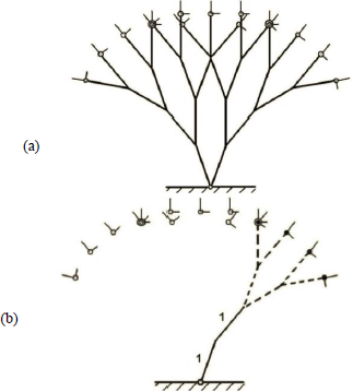
Fig. 3: (a) Illustration of all possible configurations of a BM with four R-link modules and the related end frames, (b) illustration of the sub-workspace 11--.

Figure 4 shows the second step of the solution, for a four-module binary R-link manipulator. The first module is the decided module. Its configuration is 1. The second module is the pending module. The other two modules shown by dashed lines are undecided modules. So they are assumed to be in their 'mean configuration'. The mean configuration of a module is a virtual configuration for it whose end frame is located in the mean position of the module workspace. According to the figure, choosing configuration 1 for the second module causes less distance between end frame and target frame than configuration 2. So configuration 1 is selected for the second module.

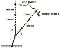
Fig. 4: The second step of Suthakorn's method for a four-module binary R-link manipulator. 1, 2 and mean illustrated in the figure correspond to configurations 1, 2 and mean, respectively.

If the number of modules is B and each module has m configurations, the number of the manipulator configurations is m^B. Accordingly, if we use a brute force method, which means evaluating all possible configurations of the manipulator in order to choose the proper configuration, then we should solve m^B forward kinematic problem. But in Suthakorn's method it is reduced to m×B.

C. The first idea: two-by-two searching

In this method, the configuration of two modules is selected in each step of the solution. If the number of the modules is odd, then in the last step, the configuration of one module is selected by Suthakorn's method. Same as Suthakorn's method, the undecided modules are assumed to be in their mean configuration. A configuration is selected for pending modules among all possible combinations of configurations, causing less distance between end frame and target frame. If the pending modules have m_i and m_j configurations at a step, then there will be m_im_j configurations which should be evaluated at that step. Pending pair modules are not necessarily adjoined and can be chosen among undecided modules arbitrarily. Accordingly, a list of modules is made in pairs, defining the pending modules for each step which is called "order list". The order of choosing the modules as pending pair modules effects on the results. Numerical results show that it is better to choose non-adjacent modules as pending modules at each step. In this paper each of the two pending modules is chosen randomly from the undecided modules of each of the two halves of the manipulator.

To clarify this method, the first step of the solution for a four-module binary R-link manipulator is shown in Fig. 5. The corresponding order list is {(1,3),(2,4)}. So the pending modules at the first step are the 1st and 3rd modules of the manipulator. At this step, the 2nd and 4th modules are undecided modules; and so are assumed in their mean configuration. According to the figure, the distance between end frame and target frame is the shortest in configuration 1-1-, where "-" is related to undecided modules. So configuration 1 is selected for both 1st and 3rd modules at this step.

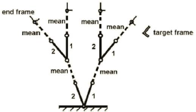
Fig. 5: First step of solution for a four-module binary R-link manipulator using two-by-two method.

D. The second idea: Iteration

In this method, at first, the two-by-two searching algorithm runs. So the configurations of all modules are defined. After that, two modules are chosen randomly among all manipulator modules. These two are considered to be pending pair modules and the others are 'decided' modules. The distance between end frame and target frame is evaluated for all possible combinations of the pending pair modules configurations. Then the configuration corresponding to the least distance is selected as the new configuration of pending modules. This process iterates by choosing two modules as pending pair modules, randomly between all manipulator modules. After that, a similar process is repeated.

The number of iterations is defined equal to the number of module pairs being chosen after the two-by-two algorithm runs. The numerical results of this method show an improvement in comparison with the middle actuation method.

E. Genetic algorithm method

To verify the proposed method of solving inverse kinematic problem for DAHMs, the numerical results of the proposed method are compared with the Genetic Algorithm (GA) method. The fitness function is the error which has the same definition as the other methods presented here.

F. Error definition

The target frames are defined by solving a forward kinematic problem of a prescribed configuration. So the problems have an exact solution and the error will be the distance between the end frame and the target frame. The distance between the two frames is expressed in Appendix A. Furthermore, for analysis convenience it is necessary to use dimensionless quantities. So the length of the manipulator in minimum actuation state is considered as the unit.

III. INVERSE KINEMATIC ALGORITHMS

Each one of the Suthakorn's, two-by-two searching and iteration methods explained above leads to an algorithm for solving the inverse kinematic problem. These three algorithms are Suthakorn algorithm, two-by-two searching algorithm and iteration algorithm; they are described below. In these algorithms, manipulator modules can be open or closed chain mechanisms. The modules of a manipulator can be dissimilar. The actuators can have two or more discrete states. The algorithms here have two separated parts: offline and online. The offline part is the same in all algorithms and is introduced below:

· Offline algorithm

1. Calculate g_jⁱ (i=1,2,...,B and j=1,2,...,m_i). g_jⁱ is the homogeneous transformation matrix of i^th module in configuration j. Also B is the number of modules and m is the number of possible configurations of i^th module. In this step of algorithm, the transformation matrix of each module in all of its possible configurations is obtained and stored. So it is necessary to solve forward kinematic of each module at first.
2. Calculate gⁱ_mid (i=1,2,...,B). gⁱ_mid is the transformation matrix of workspace mean frame of i^th module. The required formulas are presented in Appendix B.
3. Consider all modules in their mean configurations: g⁽ⁱ⁾= gⁱ_mid (i=1,2,...,B) where g⁽ⁱ⁾ is the transformation matrix of i^th module.

A. Suthakorn algorithm

· Online part:

1. Input target frame in the form of transformation matrix (g_target).
2. Select a proper configuration for i^th module (pending module). It starts with i=1 and continues to B.
   
   2.1) Calculate G_jⁱ (j=1,2,..., m_i) as follows:
   g⁽ⁱ⁾ = g_jⁱ
   G_jⁱ= g⁽¹⁾_° g⁽²⁾_° ... _° g^(B)
   where G_jⁱ is the transformation matrix of manipulator whose i^th module (pending module) is in configuration j.
   
   2.2) Calculate the distance between end frame and target frame D(G_jⁱ,g_target).
   
   2.3) Find the minimum amount of D from among all amounts calculated in the previous step (min{ D(G_jⁱ,g_target): j=1,2,...,m_i }). If the corresponding j is illustrated by J, then
   g⁽ⁱ⁾=gⁱ_J
   
   so the configuration J is selected for the i^th module.
   2.4) If i < B then i =i+1 and go to 2.1.

B. Two-by-two searching algorithm

In the following algorithm, it is assumed that the number of modules is even. For odd numbers, the last step of solution is done for one module using Suthakorn algorithm.

· Online part:

1. Input target frame in the form of transformation matrix (g_target).
2. Make order list (L). It can be done by setting the natural numbers 1 to B in a list, randomly and sorting each pair of numbers L_i (i=1,2,...,B/2) from small to big. These are expressed as follows:
   L={L₁,L₂,...,L_B/2}
   L_i=(L_i1, _i2)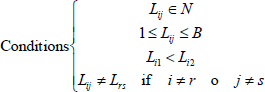
3. Select a proper configuration for pending modules L_i1 and L _i2. i starts from 1 and continues to B/2. It can be done as follows:
   
   3.1) Calculate Gⁱ_j,k (j=1,2,...,m _Li1,k=1,2,...,m _Li2) as follows:
   g^(Li1) = g_j^Li1
   g^(Li2) = g_k^Li1
   Gⁱ_j,k= g⁽¹⁾_° g⁽²⁾_° ... _° g^(B)
   where Gⁱ_j,k is the transformation matrix of manipulator which its pending modules L_i1 and L _i2 are in configuration j and k, respectively.
   
   3.2) Calculate the distance between end frame and target frame, D(Gⁱ_j,k,g_target).
   
   3.3) Find the minimum amount of D from among all amounts calculated in the previous step (min{ D(Gⁱ_j,k,g_target): j=1,2,...,m _Li1 ,k=1,2,...,m _Li2}).. If the corresponding j and k are illustrated by J and K respectively, then
   g^(Li1) = g_J^Li1
   g^(Li2) = g_K^Li1
   so the configurations J and K are selected for the L_i1^th and L_i2^th modules, respectively.
   
   3.4) If i < B/2 then i=i+1 and go to 3.1.

C. Iteration algorithm

The online part of this algorithm is divided into two parts. The first part is the two-by-two searching algorithm. The second part which iterates for prescribed times (n_itr) is expressed below:

1. i=1
2. Select R₁ and R₂ randomly, whose conditions are:
   R₁ , R₂ ∈ N
   1≤ R₁ , R₂≤B
3. Run steps 3.1 to 3.3 of the two-by-two searching algorithm where R₁ and R₂ are used instead of L_i1 and L_i2, respectively.
4. If i < n_itr then i=i+1 and go to 2.

IV. NUMERICAL RESULTS

A. Introducing the case studies

Case study 1: a 2D BM with VGT modules

A 20-module manipulator, with similar VGT modules is considered as a 2D case study. This manipulator is called "VGT manipulator". A VGT module is illustrated in Fig.6. It contains three binary prismatic actuators in AD, AC and BC links. The two other links (AB, CD) have constant lengths. A, B, C and D are passive revolute joints. This module has 2³=8 configurations. Length of constant links is 1/20. Discrete actuation amounts of binary actuators (which are the length of links AD, AC and BC) are {1/20,1.5/20}. Readers are referred to Ebert-Uphoff (1997) for forward kinematics of this module.

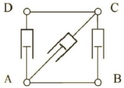
Fig. 6: A VGT module.

Case study 2: a spatial BM with 3-RPS modules

A 20-module manipulator, with similar 3-RPS modules, is considered as a 3D case study. This manipulator is called "3-RPS manipulator" in short. A 3-RPS module is shown in Fig. 7. This module is a spatial parallel robot with three binary prismatic actuators in its three legs, A₁B₁, A₂B₂ and A₃B₃. Base plate (A₁A₂A₃) and moving plate (B₁B₂B₃) are the same equilateral triangles. A₁, A₂ and A₃ are passive revolute joints whose rotation axes are parallel to their opposite sides in triangle A₁A₂A₃. B₁, B₂ and B₃ are passive spherical joints. The distances between the center and the corners of the two triangles are a=b=1/20. The discrete amounts of actuation which are the length of the legs are {1/20,1.5/20}. Readers are referred to Rao and Rao (2009) for forward kinematic of this module.

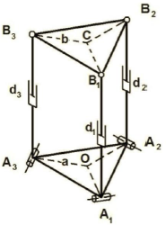
Fig. 7: A 3-RPS module.

Case study 3: a 2D DAHM with dissimilar modules

As an example of DAHMs with dissimilar modules, we simulate a 2D manipulator that is composed of R-Link and VGT module pairs cascaded one upon another continuously until we have 20 modules altogether. An R-link module is a constant link connected to the previous module by a revolute joint. Figure 1 shows a binary actuated R-link module. The actuators of R-link modules in this case study have four discrete states. The actuation amounts are {-π/9,-π/18,π/18,π/9}. So, each R-link module has four configurations. The length of the constant link is 1/20. VGT modules which are used in this case study are the same as those described in the Case study 1.

C. Numerical results

Figure 8 compares the results of the two proposed methods of inverse kinematic (two-by-two searching method and iteration method) with Suthakorn's method (Suthakorn and Chirikjian, 2001) and GA method, for case study 1 (2D, Fig. 8(a)) and case study 2 (3D, Fig. 8(b)). The target frames are obtained by solving the forward kinematic problem for some random configurations of the manipulator. It guaranties the existence of an exact solution for each sampled problem. Every value presented in Figs. 8(a) and 8(b) is an average obtained from solving 100 random sample problems. A set of real targets are used commonly for all four methods. The number of iterations in iteration method is 10. In GA method, the population size is 20; the number of generations is 100; the elite count (number of elite children which is transferred to the next population without any changes) is 2; and the crossover fraction is 0.8. All the computations were done by MATLAB software with an Intel 1.66 GHz processor.

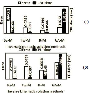
Fig. 8. a) Error and CPU-time of inverse kinematic solution of the case study 1 (2D) using four methods: Suthakorn's method (Su-M), two-by-two searching method (Tw-M), iteration method (It-M) and GA method (GA-M), b) same results for case study 2 (3D)

According to the presented results in Figs. 8(a) and 8(b), although the solution time of the Suthakorn's method is less than the other methods, its errors are high. GA method has long solution time. The two-by-two searching method and the iteration method are better than the two other methods.

Figures 9(a) and 9(b) illustrate the effect of the number of modules on error and CPU-time, respectively. These are represented for all three case studies. The results are calculated using iteration algorithm with 50 iterations. Every value in these two figures is an average of 1000 values over 1000 random samples.

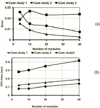
Fig. 9. The effect of the number of modules on error and CPU-time for various case studies

As Fig. 9(a) shows, the error goes down with the number of modules in 2D case studies (case studies 1 and 3) but it is not true in 3D case study (case study 2). We do not find any reason for that. As you can see in Fig. 9(b), CPU-time grows with the number of modules, almost linearly with a low slope. CPU-time of 3D case study is more than 2D case studies.

Figures 10, 11 and 12 illustrate the effect of the iterations on error and CPU-time of the case studies 1, 2 and 3, respectively. These are represented for 4, 10 and 20-module manipulators. The results are calculated using iteration algorithm with 50 iterations. Every value in these figures is an average of 1000 values over 1000 random samples.

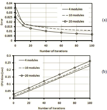
Fig. 10: Effect of iterations on (a) error and (b) CPU-time, in iteration algorithm for case study 1 (2D case: VGT manipulator)

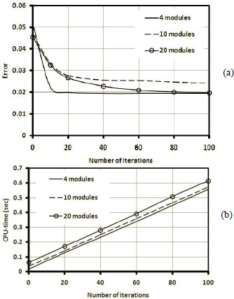
Fig. 11: Effect of iterations on (a) error and (b) CPU-time in iteration algorithm for case study 2 (3D case: 3RPS manipulator)

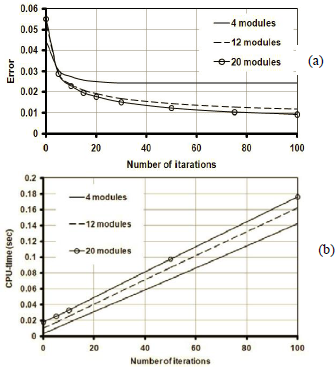
Fig. 12: Effect of iterations on (a) error and (b) CPU-time, in iteration algorithm for case study 3 (2D case with dissimilar modules)

As Figs. 10(a), 11(a) and 12(a) show, the error goes down with the number of iterations. However the reduction rate is descending and error will never be zero. According to Figs. 10(b), 11(b) and 12(b), CPU-time grows with the number of iterations, almost linearly with a low slope.

Each one of Figs. 13, 14 and 15 shows five results for five random problems, obtained by iteration algorithm with 50 iterations. Figs. 13, 14 and 15 correspond to case studies 1, 2 and 3, respectively. In these figures, the target frames are shown by dashed lines and the end frames are shown by solid lines.

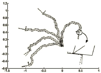
Fig. 13: Five samples of solution by iteration algorithm with 50 iterations for case study 1 (20-module VGT manipulator)

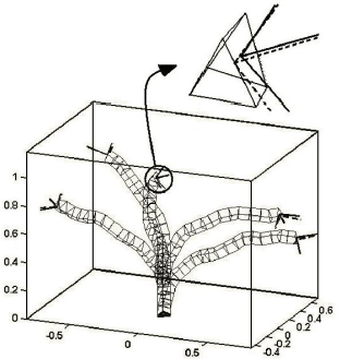
Fig. 14: Five samples of solution by iteration algorithm with 50 iterations for case study 2 (20-module 3RPS manipulator)

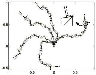
Fig. 15: Five samples of solution by iteration algorithm with 50 iterations for case study 3 (2D manipulator composed of R-link and VGT module pairs cascaded one upon another continuously until the number of modules is 20)

V. CONCLUSIONS

Two methods (two-by-two searching method and iteration method) have been proposed to modify Suthakorn's method of solving inverse kinematic problems of DAHMs. The numerical results show that these methods (especially iteration method) efficiently decrease the errors of Suthakorn's method. Furthermore they are significantly more efficient than GA method in terms of error and CPU-time. The proposed methods can not find the exact solution even after a large number of iterations.

APPENDIX A

The homogeneous transformation matrix can be expressed as follows

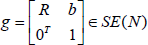(A1)

where, R∈SO(N) is the rotation matrix and b∈R^N is the position vector. N for 2D cases is 2 and for 3D is 3. The distance between two frames which are illustrated by g₁ and g₂ can be expressed as follows:

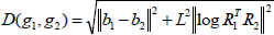(A2)

where ||.|| is the Euclidean norm. L is a parameter mainly introduced to match units of the squared terms. In this paper the value of L=0.1 was used. Readers are referred to (Park, 1995; Kyatkin and Chirikjian, 2000) for more information.

APPENDIX B

Consider a set of N homogeneous transformation matrixes. It is illustrated by {g_i=g(b_i,R_i): i=1,2,...N} where g, R and b are described in Appendix A. The mean of this set which is illustrated by g_m=g(b_m,R_m), can be calculated as follows:

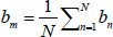	(B1)
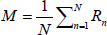	(B2)
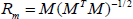	(B3)

Because M in Eq. (B2) is not included in SO(N), R_m is taken to be the closest rotation matrix to M in Eq. (B3). If g_m=g(b_m,R_m) is the homogeneous transformation matrix related to the generalized workspace mean frame of a module, the mean frame of a generalized workspace of P similar modules which is illustrated by g^*_m=g(b^*_m,R^*_m) can be evaluated as follows:

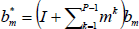	(B4)
	(B5)
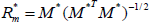	(B6)

where I is unit matrix. For 2D cases R^*_m=(R_m)^P, but it is not true for 3D cases and Eqs. (B5) and (B6) should be used. Readers are referred to Suthakorn and Chirikjian (2001) for more information.

REFERENCES
1. Chen, Q., Y. Haddab and P. Lutz, "Microfabricated bistable module for digital microrobotics," J. Micro-Nano Mech., 6, 1-12 (2011).
2. Chirikjian, G.S., and D.S. Lees, "Inverse kinematics of binary manipulators with applications to service robotics," Proc. IROS '95, Pittsburgh, 65-71 (1995).
3. Ebert-Uphoff, I., On the development of discretely-actuated hybrid-serial-parallel manipulators, Ph.D. Dissertation, Johns Hopkins University (1997).
4. Ebert-Uphoff, I., and G.S. Chirikjian, "Efficient workspace generation for binary manipulators with many actuators," J. Robot. Syst., 12, 383-400 (1995).
5. Ebert-Uphoff, I. and G.S. Chirikjian, "Inverse kinematics of discretely actuated hyper redundant manipulators using workspace densities," Proc. IEEE Int. Conf. on Robotics and Automation, 139-145 (1996).
6. Ebert-Uphoff, I. and G.S. Chirikjian, "Discretely actuated manipulator workspace generation by closed-form convolution," ASME J. Mechanical Design, 120, 245-251 (1998).
7. Kyatkin, A.B., and G. S. Chirikjian, Engineering applications of noncommutative harmonic analysis, CRC Press (2000).
8. Mohan Rao, N., and K. Mallikarjuna Rao, "Dimensional synthesis of a spatial 3-RPS parallel manipulator for a prescribed range of motion of spherical joints," Journal of Mechanism and Machine Theory, 44, 477-486 (2009).
9. Park, F.C., "Distance metrics on the rigid-body motions with applications to mechanism design," Trans. ASME, 117, 48-54 (1995).
10. Petit, L., C. Prelle, E. Dore and F. Lamarque, "Digital electromagnetic actuators array," IEEE/ASME International Conference on Advanced Intelligent Mechatronics, Montréal, Canada, July 6-9 (2010).
11. Proulx, S. and J.-S. Plante, "Design and experimental assessment of an elastically averaged binary manipulator using pneumatic air muscles for magnetic resonance imaging guided prostate interventions," Transactions of the ASME, Journal of Mechanical Design, 133, 1-9 (2011).
12. Scofano, F.S., M.A. Meggiolaro and V.A. Sujan, "Inverse Kinematics of a Binary Flexible Manipulator Using Genetic Algorithms," ABCM Symposium Series in Mechatronics v.2, Brazilian Society of Mechanical Sciences and Engineering, Rio de Janeiro, Brasil, 202-209, (2006).
13. Sujan, V.A., and S. Dubowsky, "Design of a Lightweight Hyper-Redundant Deployable Binary Manipulator," ASME Journal of Mechanical Design, 126, 29-39 (2004).
14. Suthakorn, J. and G.S. Chirikjian, "A new inverse kinematics algorithm for binary manipulators with many actuators," Adv. Robotics, 15, 225-244 (2001).

Received: July 19, 2011
Accepted: September 20, 2012
Recommended by Subject Editor: Eduardo Dvorkin