Reinforcement learning using gaussian processes for discretely controlled continuous processes

M. de Paula and E.C. Martínez

Instituto de desarrollo y diseño - INGAR (CONICET - UTN). {marianodepaula, ecmarti}@santafe-conicet.gov.ar

Abstract— In many application domains such as autonomous avionics, power electronics and process systems engineering there exist discretely controlled continuous processes (DCCPs) which constitute a special subclass of hybrid dynamical systems. We introduce a novel simulation-based approach for DDCPs optimization under uncertainty using Reinforcement Learning with Gaussian Process models to learn the transitions dynamics descriptive of mode execution and an optimal switching policy for mode selection. Each mode implements a parameterized feedback control law until a stopping condition triggers. To deal with the size/dimension of the state space and a continuum of control mode parameters, Bayesian active learning is proposed using a utility function that trades off information content with policy improvement. Throughput maximization in a buffer tank subject to an uncertain schedule of several inflow discharges is used as case study addressing supply chain control in manufacturing systems.

Keywords— Hybrid Systems; Stochastic Systems; Optimization; Reinforcement Learning (RL); Gaussian Processes (GP).

I. INTRODUCTION

Modern automated systems are often constituted by interacting components of heterogeneous continuous/ discrete nature. Dynamical systems having such a hybrid continuous/discrete nature are named hybrid systems (HS). We can find HS in electrical systems, chemical plants, biological systems, supply chains, unmanned vehicles, solar energy collectors, wind turbines and many others. A discretely controlled continuous process (DCCP) is a special type of hybrid systems where the discrete-event dynamics is the result of some event-based control strategy used to respond to external disturbances and endogenous inputs affecting the state evolution of the controlled system as whole (Simeonova, 2008; Goebel et al., 2009; Lunze and Lehmann, 2010).

A control strategy is implemented by a switching policy which timely stops an operating mode due to goal achievement, a state constraint or an external event (Mehta and Egerstedt, 2006). Each control mode, or simply "mode," implements a parameterized feedback control law until a terminating condition is activated. Then, each mode differs from other by its parameterization which varies in a continuum. Duration time for each mode execution depends on the type of behavior or specific goal which is being pursued and occurrence of disturbances and events affecting the system dynamics. For optimal control, the switching policy must generate a sequence of control modes to complete a goal-directed control task from different initial states while minimizing some performance criterion (Görges et al., 2011). Thus, optimal operation of a DCCP gives room for resorting to a Lebesgue sampling strategy of states to advantage (Xu and Cao, 2011). This paper deals with the problem of finding a switching policy for optimal operation of a DCCP under uncertainty so as to implement a goal-directed control strategy in real-time.

For a finite number of modes, a novel modeling paradigm known as integral continuous-time hybrid automata (icHA) has been recently proposed for event-driven optimization-based control for which no a priori information about the timing and order of the events is assumed (Di Cairano et al., 2009). The solution of dynamic optimization problems with continuous time hybrid automata embedded has been thoroughly reviewed by Barton et al. (2006). In a more recent work, approximate dynamic programming has been successfully applied to the discrete-time switched LQR control problem (Zhang et al., 2009). The important issue of optimality in multi-modal optimal control has also been addressed by Mehta and Egerstedt using reinforcement learning (RL) techniques regarding a finite set of control modes (Mehta and Egerstedt, 2006).

Uncertainty in the initial states is a major obstacle for multi-modal control since fixed control programs are derived from assumed initial conditions. Reinforcement Learning (RL) (Sutton and Barto, 1998) is a simulation-based approach to solve optimal control problems under uncertainty. For optimal operation of DCCPs under uncertainty a multi-modal control program should be able to adapt on-line in order to handle disturbances or events that may severely affect a control program performance or renders it even unfeasible. In this work, the main argument is that for optimal operation of a DCCP under uncertainty a switching policy is required to implement goal-directed control in real-time. A novel simulation-based algorithm which combines dynamic programming with Lebesgue sampling and Gaussian process (Rasmussen and Williams, 2006) approximation is proposed to learn a switching policy for mode selection. To deal with the size and dimension of the state space and a continuum of feedback law parameters, Bayesian active learning (Deisenroth et al., 2009) is proposed using a utility function that trades off information content with switching policy improvement. Probabilistic models of the state transition dynamics following each mode execution are learned upon data obtained by increasingly biasing operating conditions.

II. DISCRETELLY CONTROLLED CONTINUOUS PROCESSES (DCCPs)

A DCCP is composed by the five components shown in Fig. 1: the continuous dynamics , where , is the control vector and the exogenous disturbances; the event generator (EG) is made up of stopping conditions that defines the endogenous binary inputs ξ_e of the control mode, a parameterized feedback law the switching policy p(x,d) which defines a decision rule for choosing control mode parameters over time t in order to achieve a control goal G.

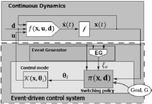
Fig. 1. Discretely Controlled Continuous Process

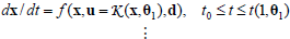
When the system operates under a certain control mode with parameter θ_i, control actions are taken using which is applied until a stopping condition ξⁱ_e∈ξ_e, i=1,...,n_e triggers changing its value from "0" to "1." Then the switching policy π must select a different θ_j. Thus, the system evolves according to:

	(1)

where t(k,θ_j) denotes the time when an endogenous binary ξⁱ_e changes its value from 0 to 1 and the control mode being executed in the kth decision stage is interrupted.

The dynamics of a DCCP under a given switching policy π is shown in Fig. 2 . The fact that execution times of control modes are different gives room for adopting a Lebesgue sampling strategy where sampling the system state is only needed when the execution of a certain mode is stopped. Thus, the system controlled under a switching policy converts the continuous time problem into an event-driven one based on stopping conditions for mode execution. The advantage of Lebesgue sampling is that it provides a finite state space which facilitates using RL algorithms. However, there is a continuum space for decision variables (control mode parameters) and the uncertainty in the mode transition dynamics makes mandatory incorporating function approximation techniques.

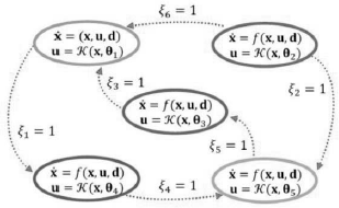
Fig. 2. Lebesgue sampled finite automaton.

III. OPTIMAL OPERATION OF DCCPs

A. Reinforcement Learning

In this section, a brief review of the RL framework (Sutton and Barto, 1998) is presented, and then, the technique of Dynamic Programming (DP) (Deisenroth et al., 2009) is used to solve the Lebesgue-sampling based optimal control problem under uncertainty. Along this work it is assumed that the mode transition dynamics is given by (1). The process dynamics is assumed initially unknown, yet it is considered to evolve smoothly over time under a given control mode.

The reinforcement learning problem consists in learning iteratively to achieve a goal (control task) from interactions with a real or simulated system. During learning, an agent (or controller) interacts with the process by execution actions (setting mode parameters) and, after that, the system evolve from the state x_k to x_k+1 and the agent receive a numerical signal τ_k called reward (or cost), that provides a measure of how good (or bad) the executed mode from x_k is in terms of observed transition. Rewards are directly related to the achievement of a sub-goal or behavior.

In applying RL to DCCPs the objective of the agent is learning the optimal policy for timely mode switching, π*, which defines the optimal mode parameters for any state the system may be in bearing in mind both short-and long term rewards. To this aim, the learning agent executes a sequence of modes to maximize the amount of reward received from an initial state/ disturbance pair (x₀,d₀) until a certain goal state is reached. Under a given switching policy π, let's assume the expected cumulative reward or value function over a certain time interval is a function of (x^π,d^π, t^π,q^π), where are the time instants at which mode switches occur. are the corresponding state values, are the corresponding disturbance values and defines the policy-specific sequence of control modes. The sequence x^πof state transitions gives rise to rewards which are used to define a discounted value function

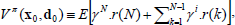(2)

where γ∈(0,1] is the discount factor which weights future rewards. An optimal policy π^* for the N-mode control problem maximizes Eq. (2) for any initial state x₀. The associated state-value function satisfies the Bellman's equation:

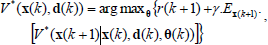(3)

The control value function Q^* is defined by

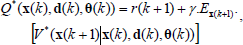(4)

such that 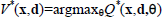for all (x,d). Once Q^* is known through interactions, then the optimal switching policy obtained directly through:

(5)

To find the Q^*-values for alternative parameterization of control modes the well known Dynamic Programming for policy iteration can be used. DP algorithms are obtained by turning the Bellman equation into update rules for improving approximations of the desired value functions. Using DP the optimal state-mode function V^* is obtained by the well-known DP recursion:

(6)

for all states x_k and k=N−1,...,0. To apply DP a number of issues must be addressed. First, the transition dynamics f must be known. Also, the state space X and mode parameter space Θ must be arbitrarily discretized. Finally, the search for the optimal policy must sample X by selectively leading the system from an initial state to the goal state requiring only a small number of interactions with the real system. For this reason, a function approximating technique is needed to have a compact representation of value functions and state transition dynamics.

Inductive modeling using function approximation can be classified into two main types: parametric and non-parametric regression. Parametric regression using for instance polynomials, radial basis functions and neural networks requires choosing a model structure beforehand. The major drawback of resorting to parametric approximation of value functions in RL is that the model class is maintained as new data from interactions are obtained. Moreover when the size of the training set is small, is often the case that value function approximation is unreliable to say the least. Nonparametric regression is far more flexible and the model structure is also changed as the dataset increases. Nonparametric regression does not imply that fitted models are parameters-free, but instead that the number of parameters and their values are simultaneously learned based on available data. Gaussian Process (GP) models are a powerful tool to deal with this type of problems. A Gaussian Process is a generalization of a Gaussian probability distribution where the distribution is over functions instead of stochastic variables.

B. Gaussian Processes

In the following, a brief introduction to GPs will be given based on the books by Rasmussen and Williams Rasmussen and Williams, 2006) using the value function V_k^*(·) as a representative example. Given a data set {Z_k,V_k} from previous interactions with a DCCP and consisting of visited state/disturbance pairs z(k)=(x(k), d(k))∈Z_k and the corresponding estimation of their values V_k^*, we want to infer an inductive model h of the (unknown) value function V_k^*(·) that generated the observed data. Thinking that the observations are generated by within a Bayesian framework, the inference of the underlying function h is described by the posterior probability

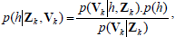(7)

where p(V_k|h,Z_k) is the likelihood and is a p(h) a prior on plausible value functions assumed by the GP model. The term p(V_k|Z_k) is called the evidence or the marginal likelihood. When modeling value functions in RL using GPs, a GP prior p(h) is placed directly in the space of functions without the necessity to consider an explicit parameterization of the approximating function h. This prior typically reflects assumptions on the, at least locally, smoothness of h.

Similar to a Gaussian distribution, which is fully specified by a mean vector and a covariance matrix, a GP is specified by a mean function m(·) and a covariance function also known as a kernel. A GP can be considered a distribution over functions. However, regarding a function as an infinitely long vector, all necessary computations for inference and prediction of value functions can be broken down to manipulating well-known Gaussian distributions. The fact that the value function V_k^*(·) is GP distributed is indicated by 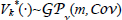hereafter.

Given a GP model of the value function V_k^*(·), we are interested in predicting the value function for an arbitrary input z_k^*. The predictive (marginal) distribution of the value function approximation for a test input z_k^* is Gaussian distributed with mean and variance given by:

	(8)
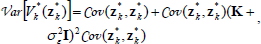	(9)

where K is the kernel matrix with 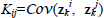. A common covariance function is the squared exponential (SE):

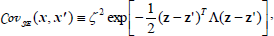(10)

where 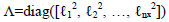and being the characteristic length scales. The parameter z² describes the variability of the inductive model h. The parameters of the covariance function are the hyper-parameters of the and collected within the vector Ψ.To fit parameters to value function data the evidence maximization or marginal likelihood optimization approach is recommended (see Rasmussen and Williams, 2006, for details). The log-evidence is given by:

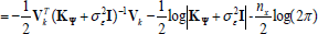	(11)

In Eq. (11), 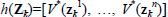where n is the number of training points. We made the dependency of K on the hyper-parameters Ψ explicit by writing K_Ψ in Eq. (11). Evidence maximization yields an inductive model of the value function that (a) rewards data fitting, and (b) rewards simplicity of the model. Hence, it automatically implements Occam's razor, i.e. preferring the simplest hypothesis (model).

C. Learning algorithm for mode switching

Assuming that the continuous dynamics evolve smooth-ly while a given control mode is implemented, learning a switching policy through interactions demands learning also the transition dynamics. We implicitly assume that output variability is due to uncertainty about stopping conditions activation. Due to the uncertainty about the resulting state due to a mode execution, a GP is used for inductive modeling state/disturbance transitions. Thus, the dynamics GP, is used to describe the state/ disturbance transition dynamics. For each output dimension d, a separate GP model is trained in such a way the effect of uncertainty about in which state the system may be in when stopping condition triggers is modeled statistically:

(12)

where m_d is the mean function, Cov_d is the covariance function. The training inputs to the transition dynamics GPs are (z,θ) pairs whereas the targets are the state differences in Eq. (12).

To learn an optimal policy we propose in this work the novel mGPDP algorithm which is based on Gaussian process dynamic programming (GPDP) (Deisenroth et al., 2009) through incorporating the use of modes to the basic GPDP algorithm based on a mode-based abstraction. GPDP describes the value functions in DP iterations directly in function space by representing them using fully probabilistic GP models that allow accounting for uncertainty in dynamic optimization. A sketch of the mGPDP algorithm using transition dynamics and Bayesian active learning for data selection is given in Fig. 3. It is worth noting that mGPDP is definitively superior to the multi-modal learning algorithm proposed in (Mehta and Egerstedt, 2008) since the entire state space may be explored. However, by means of Bayesian active learning only the most promising states are visited during learning.

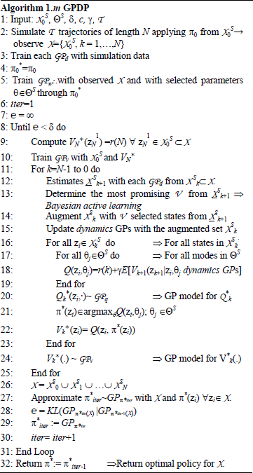
Figure3. mGPDP algorithm

The algorithm mGPDP starts from a small set of initial input locations to generate the set of reachable states Χ. Using Bayesian active learning (line 13), new locations (states) are added to the current set at any stage k. Support sets serve as training input locations for both the dynamics and the value function At each time step k, the dynamics GP is updated (line 15) to incorporate most recent information. Furthermore, the GP models for the value functions and are also updated. After each mode is executed the function r(k) is used to reward the transition. A key idea in the algorithm mGPDP is that the set is a support set of reachable states based on Lebesgue sampling. As a result, X is the set of all states that are reachable from given initial states using a sequence of modes of length less than or equal to N. For example, is a set of observable states from which the goal state can be achieved by executing only one mode. Lebesgue sampling is far more efficient than Riemann sampling which uses fixed time intervals for control. As switching policies in successive iterations are also modelled using GPs, policy iteration can be stopped when the Kullback-Leibler (KL) distance between two successive policy distributions is lower than a tolerance d. It is noteworthy that the resulting optimal switching policy π^* can be implemented on-line for unseen states

4. CASE STUDY

A. Problem Statement

As a representative case study, let's consider a hybrid dynamical system made up of two tanks in series and a five on-off taps intermittently discharging inflows into the upper tank (the smoother) as shown in Fig. 4.

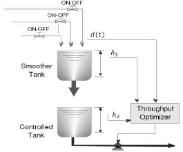
Fig. 4. Two-tank system with stochastic loading.

The smoother tank discharges its content to the controlled tank following the Torricelli's law. In the controlled tank, the control task is to maximize the average outflow rate while avoiding sudden changes whereas overflowing or emptying the tank are heavily penalized events. What makes this optimizing control task challenging is that there exists an unknown stochastic pattern for tap opening and closing. In Fig.5, a nominal realization of the discharge schedule is shown. The corresponding overall inflow rate to the smoother tank is shown in Fig. 6. As there is no control available in the upper tank, the capacity of the controlled tank must be properly managed despite uncertainty and variability.

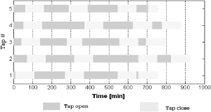
Fig. 5. Nominal discharge schedule for 5 taps

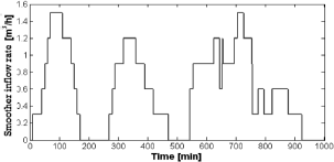
Fig. 6. Inflow rate to the upper tank

Each buffer tank has a volume of 1 m³ and the maximum level allowable is 1 m. At any time the system state is defined by the number of open taps that are discharging, tank levels in both tanks, and the actual inflow rate to the controlled tank. The controlled tank outflow discharged downstream is varied using the feedback law:

(13)

where r is the control mode parameter, h₂(t) is the instantaneous level in the controlled tank and is its exponentially smoothed level defined by:

(14)

The algorithm mGPDP has been applied to determine an optimal switching policy that maximize the plant throughput by rewarding mode transitions in such a way that the average outflow rate () is maintained as high as it is possible without overflowing or interrupting the discharge downstream. Also, sudden changes to the outflow rate (ΔF) are heavily penalized to prevent such undesirable events especially when the modes switches. Then, the reward function is designed according to Eq. (15) such that, following a mode execution, the corresponding immediate reward r(k) is calculated as:

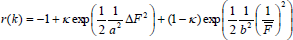(14)

whenever and r(k)=0, otherwise. is the average flow rate for the mode, ΔF is the net change in the outflow rate when the modes switches, whereas reward function parameters are: k=0.7; a=1/12; b=5. All control modes are stopped whenever a tap is open or closed. The reward function in Eq. (15) makes possible a smooth tank operation and prevents sudden outflow changes due to the modes switches while maximizing throughput.

B. Results

In Fig. 7, results obtained when the optimal switching policy obtained using the mGPDP algorithm is used to vary the flow rate downstream assuming the nominal discharge schedule. For training, the learning system was presented with schedules that were stochastic variations of the nominal schedule in Fig. 5. To generate such schedule variability, times for valve opening and closing were obtained by sampling from triangular distributions such that their mean values correspond to the nominal scheduling times, whereas the maximum and minimum values of each distribution were obtained by adding and subtracting 15 min from the corresponding nominal values. In Fig. 7 and Fig. 8, results obtained for the controlled tank under the nominal schedule which has not been used for training. As can be seen by varying mode parameter the multi-modal controller is able to handle appropriately the nominal schedule of on-off discharges from the taps by changing the parameter θ.

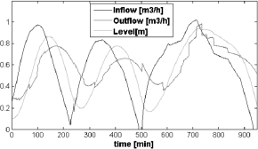
Fig. 7. Multi-modal control for the nominal schedule

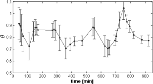
Fig. 8. Mode switching for the nominal schedule

To address the robustness of the learned switching policy we take a testing schedule which is a significant variation of the nominal schedule in Fig. 5. Figure 9 depicts the inflow rate to the smoother tank associated with the schedule used for testing. As can be seen, the discharge pattern from taps is noticeable different from the nominal schedule shown. In Fig. 10, the controlled and manipulated variables for the lower tank when the switching policy is applied are shown. Finally, in Fig. 11 the sequence of control mode parameters during testing are given. It is worth noting that the uncertainty for the mode parameter θ at each switching time is quite low despite the difference between tap schedules.

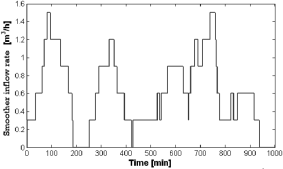
Fig. 9. Smoother inflow rate for the testing schedule

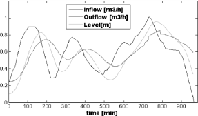
Fig. 10. Switching control for the testing schedule

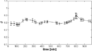
Fig. 11. Mode switching for the testing schedule

V. FINAL REMARKS

From supply chains to hybrid chemical plants, from bioprocesses and biological systems to solar collectors and wind turbines are all representative examples of a special type of hybrid dynamical systems known as DCCPs. For optimal operation under uncertainty, timely switching to different control modes is necessary. A novel integration of dynamic programming with Gaussian Processes using modes has been proposed to determine an optimal switching policy. Data gathered over a number of simulated interactions with the system is used to learn a regression metamodel of the transition dynamics which is instrumental in making the proposed algorithm mGPDP ideal for both learning via intensive simulation the switching policy and adapting it to the true operating environment a DCCP is facing over time.

REFERENCES
1. Barton, P.I., C.K. Lee and M. Yunt, "Optimization of hybrid systems," Computers and Chemical Engineering 30, 1576-1589 (2006).
2. Di Cairano, S., A. Bemporad and J. Júlvez, "Event-driven optimization-based control of hybrid systems with integral continuous-time dynamics," Automatica, 45, 1243-1251 (2009).
3. Deisenroth, M.P., C.E. Rasmussen and J. Peters, "Gaussian process dynamic programming." Neurocomputting, 72, 1508-1524 (2009).
4. Goebel, R., R. Sanfelice and A. Teel, "Hybrid dynamical systems," IEEE Control Systems Magazine, 29, 28-93 (2009).
5. Görges, D., M. Izác and S. Liu, "Optimal Control and Scheduling of Switched Systems," IEEE Transactions on Automatic Control, 56, 135-140 (2011).
6. Lunze, J. and D. Lehmann, "A state-feedback approach to event-based control," Automatica, 46, 211-215 (2010).
7. Mehta, T.R. and M. Egerstedt, "An optimal control approach to mode generation in hybrid systems," Nonlinear Analysis, 65, 963-983 (2006).
8. Mehta, T.R. and M Egerstedt, "Multi-modal control using adaptive motion description languages," Automatica, 44, 1912-1917 (2008).
9. Rasmussen, C.E. and C.K.I. Williams, Gaussian processes for machine learning, MIT Press (2006).
10. Simeonova, I., On-line periodic scheduling of hybrid chemical plants with parallel production lines and shared resources, Master's Thesis, Université catholique de Louvain (2008).
11. Sutton, R.S. and A.G. Barto, Reinforcement learning: an introduction, MIT Press (1998).
12. Xu, Y.-K. and X.-R. Cao, "Lebesgue-Sampling-Based Optimal Control Problems With Time Aggregation," IEEE Transactions on Automatic Control, 56, 1097-1109 (2011).
13. Zhang, W., J. Hu and A. Abate, "On the Value Functions of the Discrete-Time Switched LQR Problem," IEEE Transactions on Automatic Control, 54, 2669-2674 (2009).

Received: May 3, 2012
Accepted: October 17, 2012
Recommended by Subject Editor: Gastón Schlotthauer, María Eugenia Torres and José Luis Figueroa