Linear algebra and optimization based controller design for trajectory tracking of typical chemical process

M.E. Serrano^†*, G. J. E. Scaglia^†, P. Aballay^†, O.A. Ortiz^† and V. Mut^‡

^† Instituto de Ingeniería Química, Universidad Nacional de San Juan, Argentina
^‡ Instituto de Automática, Universidad Nacional de San Juan, Argentina
^* Corresponding author. Tel. +54-264-421-1700; Fax. +54-264-422-7216.
Email: eserrano@fi.unsj.edu.ar, {gscaglia, paballay, rortiz} @unsj.edu.ar, vmut@inaut.unsj.edu.ar

Abstract— This paper presents a new controller design to tracking trajectory of a typical chemical process. The plant model is represented by numerical methods and, from this approach; the control actions for an optimal operation of the system are obtained. Its main advantage is that the condition for the tracking error tends to zero and the calculation of control actions, are obtained solving a system of linear equations. The proofs of convergence to zero of the tracking error are presented. Simulation results show the good performance of the proposed control system.

Keywords— Control System Design, Nonlinear Model, Tracking Trajectory Control, Numerical Methods, Typical Chemical Process.

I. INTRODUCTION

The control of liquid level in tanks and flow between tanks is a basic problem in the process industries. The process industries require liquids to be pumped, stores in tanks and then pumped to another tank. An example is the fermentation process with different microorganisms in the biotechnology industry. Chung et al. (2005) show some applications, it suggests that periodic operations can give results where the yield and selectivity can improve or make possible the continuous operation. To control liquid level the traditional method PID control is used due to its reliability, simple structure and easy parameters adjust (Tunyasrirut et al., 2006; Gou, 2008, and Liu, 2004). To perform high precision liquid level control and good tracking precision in the presence of the system nonlinearities, it is needed to use nonlinear control method to solve these problems effectively and achieve precise control. Neural network (Hou, 2009; Huang and Chiou, 2006) and genetic algorithm (Tan and Li, 2001; Moshir et al., 2003) based controllers are proposed as effective tools for nonlinear controller design. Limon et al. (2010) applies tracking techniques to track processes consisting of four tanks which form a multivariable nonlinear system. They pose a technique based on MPC (model predictive control based on the model) where the plant model is assumed as a linear system with bounded uncertainty to a polyhedral set known, under this assumption the proposed controller is feasible in any changes to the set points and leads the system at this point whenever possible. If the goal is not permissible, therefore unreachable, the system is directed to the nearest point allowable operating. Usually, in literature the goal is find the control actions that combined, result in tracking a desired trajectory.

This paper provides a positive answer to the previous challenging problem.

In this work a trajectory-tracking controller, designed originally for robotic systems Scaglia et al. (2009) is applied for trajectory tracking of the four tanks plant (Limon et al., 2010). This simple approach suggests that knowing the value of the desired state, it can find a value for the control action, which forces the system to move from its current state to the desired one. The main contribution of this work is that the proposed methodology is based upon easily understandable concepts, and there is no need of complex calculations to attain the control signal.

Another contribution of this paper is the application of Monte Carlo (MC) based sampling experiment in the simulations. The controller parameters can be computed to minimize a cost index, here being determined by the Monte Carlo (MC) experiment, and the theoretical results are validated by simulations. It's important to remark that MC experiment can be implemented on line in a real plant.

It is noteworthy that due to the above mentioned characteristics, the computing power required to perform the mathematical operations is low. Thence it is possible to implement the algorithm in any controller with low computing capacity. Furthermore, the developed algorithm is easier to implement in a real system because the use of discrete equations allows direct adaptation to any computer system or programmable device running sequential instructions at a programmable clock speed. Thus, among the main advantages of this approach are the simplicity of the controller and the use of discrete-time equations, simplifying its implementation on a computer system. The proof of the zero-convergence of the tracking error is another main contribution of this work.

The methodology developed for tracking the desired trajectory (h_1d and h_2d) is based on determining the desired trajectories of the remaining state variables. These variables states are determined through analyzing the conditions for a system of linear equations to have an exact solution. Therefore, the control signals are obtained by solving the system of linear equations. In addition, to complete the previous work of the authors (Scaglia et al., 2009), the proof of the zero-convergence of the tracking error is included in this paper.

The paper is organized as follows: in section 2, the dynamic model of the four tanks plant is presented. The methodology of the controller design is show in section 3. In Section 4, the theoretical results are validated with simulation results of the control algorithm. Finally, Section 5 presents the conclusions and some topics that will be addressed in future contributions.

II. METHODOLOGY FOR CONTROLLER DESIGN

A. Model of the Four Tanks Plant

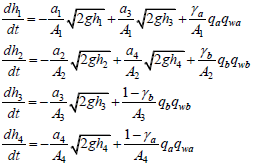
The four tanks plant is a multivariable laboratory plant of interconnected tanks with nonlinear dynamics. A state-space continuous time model of the quadruple-tank process system (Limon et al., 2010) can be derived from first principles as follows

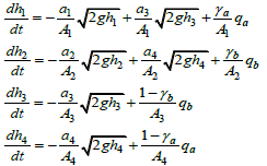(1)

The state variables are h₁ level of tank 1, h₂ level of tank 2, h₃ level of tank 3, and h₄ level of tank 4. The control objective is to find the values of the flows into (q_a and q_b) so that the variables h₁ and h₂ follow with a minimum error the preset trajectories h_1d and h_2d respectively.

B. Problem Statement

Let us consider the first-order differential equation,

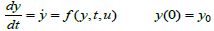(2)

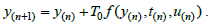
where y represents the output to the system to be controlled, u the control action, and t the time. The values of y(t) at discrete time t=nT₀, where T₀ is the sampling period and will be denoted as y_(n). Thus, when computing y_(n+1) by knowing y_(n), Eq. (2) should be integrated over the time interval as follows:

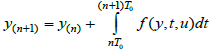(3)

where, u remains constant during the interval 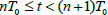. There are several numerical integration methods to calculate y_(n+1). For instance, the Euler method approaches can be used,

(4)

The use of numerical methods in the simulation of the system is based mainly on the possibility to determine the state of the system at instant n+1 from the state, the control action, and other variables at instant n. So, y_(n+1) can be substituted by a function of reference trajectory and then the control action to make the output system evolve from the current value (y_(n)) to the desired one, can be calculated. Therefore, if it is known beforehand the desired trajectory (referred to as y_d(n+1)) to be followed by y(t), then y_(n+1) can be substituted by y_d(n+1) into Eq. (2), thus is possible to calculate u_(n). It represents the control action required to go from the current state to the desired one.

To accomplish the previous achievement, it is necessary to solve a system of linear equations for each sampling period, as shown in next Section. This represents an important advantage mainly for two reasons, first for complex systems (linear or nonlinear), the equations can be solved using iterative methods for solving systems of linear equations, which only need an initial value to start the iteration. This value may be precisely the estimate calculated in the previous sampling instant. Second, this methodology can be applied to other types of systems and the accuracy required by the numerical method is less than the one needed to simulate the behavior of the system under study. This is because, when state variables are available for feedback, at each sampling instant, the method corrects any differences caused by the cumulative error (for example, "rounding errors"). So, the approximation is used to find the best way to go from one state to the next, according to the availability of the system model.

In this paper we propose to apply this approach in the dynamic model of the four tanks plant and thus obtain the control actions that allow to the system follow a trajectory previously established. In the next section, the design of the proposed controller will be analyzed.

C. Controller Design

In this section, is designed a control law capable of generating the signals , that allow to variables h₁ and h₂ follow the desired trajectory, h_1d and h_2d respectively.

The Eq. (1) can be expressed as follow,

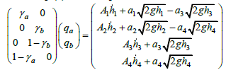(5)

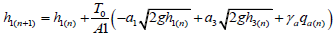
When using the Euler approximation in (5), we have:

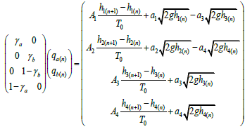(6)

The numerical methods can be used to calculate the evolution of the system. This is, that the system state at time n+1 can be determined knowing the states and control actions at time n. Thus it is possible to calculate the control actions so that the system moves from the current state to desire. Then, considering (6) and the numerical methods is proposed the following system of linear equations:

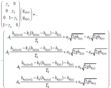(7)

or, in compact form as.

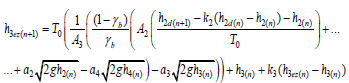
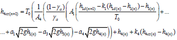
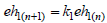
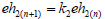
(8)

In (7), h_4ez and h_3ez are the reference values that to be taken by variables h₃ and h₄ respectively for the variables h₁ and h₂ follow the desired values. The controller parameters k₁, k₂, k₃ and k₄ allows the tracking error tends to zero, they satisfied that: 0<k₁0<1, 0<k₂<1, 0<k₃<1 and 0<k₄<1, (see Appendix). Now, the goal is to find q_a(n) and q_b(n) such that the trajectory tracking error tend to zero. To accomplish this, the system (8) must have exact solution. Then the vector b must be contained in the space formed by the columns of A, i.e., the vector b must be linear combination of the column vectors of matrix A (Strang, 1980; Scaglia et al., 2009).

As can be seen in (7), a proportional action (k₁, k₂, k₃ and k₄) to the error is considered in the computation of the control inputs.

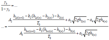
Then, by analyzing the conditions for the system of linear equations (7) has exact solution, we obtain:

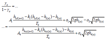	(9)
	(10)

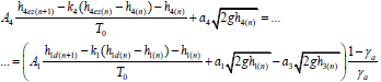
Then, from (9) and (10) so that the system (7) has exact solution can be established the following conditions:

	(11)
	(12)

The Equations (11) and (12) represent the conditions so that the system (7) has exact solution, and the tracking error tends to zero. Finally, the optimal solution of Eq. (7) is obtained by solving the normal Eq. A^TAx = A^Tb (Strang, 1980.

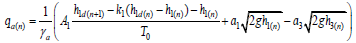
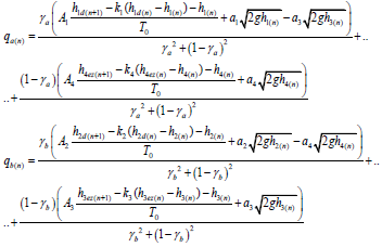(13)

The Eq. (13) represents the calculation of control actions to be applied, in the complete model expressed in (1), at time n. These make that the tracking error tends to zero (see Appendix A).

II. SIMULATIONS RESULTS

In this Section, the effectiveness of the proposed control law will be verified by simulation. The simulation conditions and the respective results will be developed below. In order to perform realistic simulations two tests were carried out using the Monte Carlo (MC) experiment (Auat Cheein et al., 2013).In the first test are perform 1000 simulations (N = 1000) and it is show how to choose the controller parameters when disturbances in control actions are considered. The second test shows the performance of the controller when considering modeling errors.

The model parameters and the considered intervals of admissible variation of the levels are obtained from Limon et al. (2010). The sampling time T₀ is 0.3 (h) and the initial conditions are h₁₍₀₎= h₂₍₀₎= h₃₍₀₎= h₄₍₀₎=0.

In the first test disturbance in the control actions are considered and the Monte Carlo experiment was carried out. To test the performance of the proposed controller the following desired trajectory is chosen,

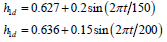The 1000 simulations are performed using MatLab software platform and in each simulations the controller's parameters are chosen considering Eq. (14),

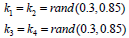(14)

where rand(0.3,0.85) is a random value with a magnitude of 0.85 and 0.3 lower bound, and rand(0.5,0.85) is a random value with a magnitude of 0.85 and 0.5 lower bound.

An additional objective of the MC experiment is to find the parameter values optimizing a defined cost function C^Φ. An idea widely used in the literature is to consider the cost incurred by the error as proposed in Batavia et al. (2002). The cost function can be represented for the combination of quadratic error in h₁ and h₂, as shown in (15).

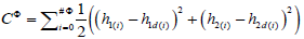(15)

where is the number of points of the trajectory. Thus, the objective is to find k₁ and k₂, in such way that C^Φ is minimized. An extra goal is demonstrate the performance of the controller against environmental disturbances. Thus, disturbance in control actions were consider:

(16)

The disturbances q_wa and q_wb are given by:

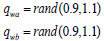(17)

where rand(0.9,1.1) is a random value with a magnitude of 1.1 and 0.9 lower bound.

Simulation results are plotted in Fig. 1 and Fig. 2. The trajectory tracking of h₁ and h₂ variables versus time along with their respective desired values (h_1d and h_2d) are shown in Fig. 1 and Fig. 2. The tracking errors are shown in Fig. 3 and Fig. 4. The Fig. 5 shows the trajectory cost obtained for the 1000 iterations. By inspection of Fig. 5 the minimum trajectory cost is C^Φ = 2.079 and is obtained in iteration #958. This cost was obtained when the controller's parameters are given by (18) and will be used in the next test.

(18)

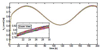
Figure 1- Tank 1 Level vs. Time.

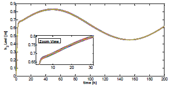
Figure 2- Tank 2 Level vs. Time.

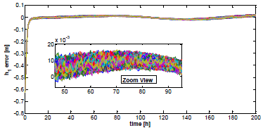
Figure 3 - Tank 1 error vs Time.

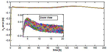
Figure 4 - Tank 2 error vs Time.

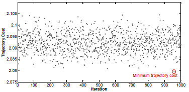
Figure 5- Trajectory cost vs. Iteration.

The Fig. 6 show the trajectory tracking when the controllers parameters are given by (18) and the minimum trajectory cost is obtained.

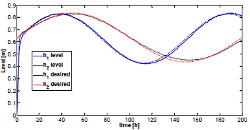
Figure 6 - Tank level vs Time, for iteration #369.

Figures 1 and 2 shows as the plant reaches the desired trajectory quickly and then continues without undesirable oscillations. Figures 3 and 4 show how the tracking error tends to zero, this convergence can also be seen in Fig. 1 and 2. The Fig. 3 shows how all the tracking errors are small despite the perturbations.

In the second test the behavior of the controller is shown with the presence of modeling errors that have not been taken into account in the controller design.

We introduce a determined error in the model parameters (above and below their nominal values) and perform 1000 simulations (N = 1000). In each simulation the controller parameters are chosen in a random way by MC based sampling. It is observed that the performance of controller designed with the technique proposed in this paper, remains very satisfactory in the following ranges of variation:

This range of variation represents the 30% of the nominal value (0.06m²).

The MC experiment was performed with a desired trajectory formed by set points. Thus, the performance of the system, when the speed of the desired trajectory changes abruptly, can be analyzed. The reference trajectory and the initial conditions are obtained from Limon et al., 2010. The values of the controller parameters are given by (18) and the sample time used is T₀ is 0.3 (h).

For 1000 iterations and whit these parametric uncertainties, the system response and the tracking error can be seen in Fig. 7 and 8, respectively. It is possible to see that the performance in the variables (h₁, h₂) is quite acceptable despite the modeling errors.

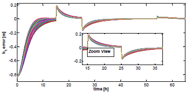
Figure 7- Tank 1 error vs. Time.

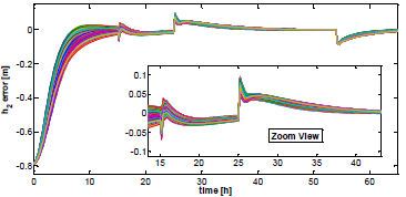
Figure 8- Tank 2 error vs. Time.

When the desired trajectory suddenly changes its direction, it is sensible to expect a momentarily increase of the error and then a decrease.

V. CONCLUSIONS

A new controller design for trajectory tracking of the Four Tanks Plant has been presented. The methodology is based on the search for conditions for which the system of linear equations has exact solution. These conditions determine the desired values of certain state variables and the control actions for the tracking error tend to zero, as shown in Appendix. If it has the process model, it only needs the values of the desired trajectory for calculating the control signals. The proposed controller has been successfully applied to the quadruple-tank process, which is a continuous nonlinear uncertain multivariable process. Furthermore, this methodology can be extended to other linear and nonlinear systems.

Simulations results are shown in this paper. The controller parameters are found by using MC method, next with these parameters, new simulations results were found. The proof of zero convergence of tracking errors developed in Appendix A demonstrates the effectiveness of the proposed methodology. This demonstration completes the previous work of the authors (Scaglia et al., 2009). The possibility to include experimental results and the saturation of the control signals in the formulation of the problem will be addressed in future contributions.

APPENDIX

If the process behavior is ruled by (7) and the controller is designed by (13), then, the tracking error when the trajectory tracking problems are considered.

The proof of convergence to zero of the tracking errors is started with the variable h₁. Then, for the system (7) has exact solution must meet (9) and (10). Considering, Eq. (9),

(A.1)

Replacing (A.1) in the control action q_a(n) corresponding to Eq. (13) and operating,

(A.2)

From the corresponding equation of the system (7),

(A.3)

Then, replacing (A.2) in (A.3) and operating,

(A.4 )

Then, operating

(A.5)

From (A.5),

(A.6)

Finally, how 0<k₁<1, then eh_1(n+1) tends to zero when .

In similar way the above analysis is applied to h₂ , h₃ and h₄, and (A.7), (A.8) and (A.9) are obtained,

	(A.7)
	(A.8)
	(A.9)

For Eq. (A.7) the controller parameter fulfills 0<k₂<1, then eh_2(n), . Considering (A.8), how 0<k₃<1, then eh_3(n+1) tends to zero when . Next, how 0<k₄<1, then eh_4(n+1) tends to zero when .

Then from (A.6), (A.7), (A.8) and (A.9), . Finally, it demonstrated that when , and the tracking error tends to 0.

REFERENCES
1. Auat Cheein F.A., F.M. Lobo Pereira, F. di Sciascio and R. Carelli, "Autonomous simultaneous localization and mapping driven by Monte Carlo uncertainty maps-based navigation," The Knowledge Engineering Review, 28, 35-57 (2013).
2. Batavia, P.; S. Roth and S. Singh, "Autonomous coverage operations in semi-structured outdoor environments," IEEE Int. Conf. on intelligent Robots and Systems, Lausame, Switzerland, 1, 743-749 (2002).
3. Chung, Y.-C., I.-L. Chien and D.-M. Chang, "Multiple-model control strategy for a fed-batch high cell-density culture processing," Journal of Process Control, 16, 9-26 (2005).
4. Gou, W., Research of intelligent PID and its applicationin the water level control, Ms.C. Thesis, Anhui Agricultural University (2008).
5. Hou, T., "Experimental Research on Neural Network PID Control Based on Hydraulic Pressure of 2-Container Water Tank," Journal of Lanzhou Jiaotong University, 28, 41-43 (2009).
6. Huang S. J. and K. C. Chiou, "An Adaptive Neural Sliding Mode Controller for MIMO Systems," Journal International Robot System, 46, 285-301 (2006).
7. Limon D., I. Alvarado, T. Alamo and E.F. Camacho, "Robust tube-based MPC for tracking of constrained linear systems with additive disturbances," Journal of Process Control., 20, 248-260 (2010).
8. Liu, K., Advanced PID control and MATLAB simulation, Publishing House of Electronics Industry (2004).
9. Moshiri, B., M. Jalili-Kharaajoo and F. Besharati, "Application of Fuzzy Sliding Mode Based on Genetic Algorithms to Control of Robotic Manipulators," IEEE Emerging Technologies and Factory Automation, 2, 16-19 (2003).
10. Scaglia, G.J.E., O.L. Quinter, V. Mut and F. di Sciascio, "Numerical Methods Based Controller Design for Mobile Robots," Robotica, 27, 269-279 (2009).
11. Strang, G., Linear Algebra and its Applications," Academic Press, New York (1980).
12. Tan, K.C. and Y. Li, "Performance-based control system design automation via evolutionary computing," Engineering Applications of Artificial Intelligence, 14, 473-486 (2001).
13. Tunyasrirut, S., T. Suksri, A. Numsomran, S. Gulpanich and K. Tirasesth, "The Auto-Tuning PID Controller for Interacting Water Level Process," Proceedings of World Academy of Science, Engineering and Technology, 12, 134-138 (2006).

Received: March 24, 2013
Accepted: March 20, 2014
Recommended by Subject Editor: José Guivant