Empirical search and characterization of contemporaneity using breaks and regime switching^°

Búsqueda empírica y caracterización de contemporaneidad utilizando quiebres estructurales y cambios de régimen

Fernando Delbianco^* - Andrés Fioriti^*

^* Department of Economics, UNS, Bahía Blanca, Argentina. Email: fernando.delbianco@uns.edu.ar, andres.fioriti@uns.edu.ar.

enviado: 23 febrero 2017
aceptado: 12 junio 2017

Abstract
This paper describes a technique to determine the contemporaneity of two economic events. It is also possible to determine some characteristics of the contemporaneity, as a descriptive stage previous to causality analysis and model estimations. As an illustration, a case of contemporaneity between news and volatility in financial markets is shown. The main result of the exercise is a Laffer curve relationship between corruption and volatility given news.

Jel Code: C13, C52, G14.

Keywords: Structural Breaks; Regime Switching; Contemporaneity and Market Volatility.

Resumen
El presente trabajo describe una nueva técnica para determinar la contemporaneidad de dos eventos económicos. Luego de ello es posible determinar algunas características de la contemporaneidad, siendo esta metodología un análisis descriptivo previo a considerar causalidad y estimar un modelo. Como ilustración, analizamos un caso de contemporaneidad entre noticias y volatilidad en mercados financieros. El principal resultado es una curva de Laffer para representar la relación entre corrupción y volatilidad dadas las noticias.

Código JEL: C13, C52, G14.

Palabras clave: Quiebres Estructurales; Cambio de Régimen; Contemporaneidad y Volatilidad de Mercados.

INTRODUCTION

Often researchers face questions to determine the correct model specification. Among those questions, an important one is to determine the relationships to study (i.e. whether the variables are dependent or controls).

Particularly, when working with breaks some relevant papers are de Peretti and Urga (2004), Harvey et al. (2001), Pesaran and Timmerman (2004) and Busetti and Harvey (2001, 2003). These papers describe the combined usage of break detection and regime estimations to find and characterize the relationship between the series under study.

One key concept on this paper is contemporaneity. The concept relies on the idea that the occurrence of breaks in one temporal series is accompanied with breaks (prior or posterior) on another series. This contemporaneity is defined by a window of time, depending on the criterion of the researcher and the nature of the data. The focus of this analysis is a-theoretical, as a first approach for a descriptive analysis, similar in concept to Granger causality tests (Granger, 1969). The methodology consists on estimating the breaks of the series and looking for contemporaneity between those breaks and periods when there was a state switch, obtaining those periods using Markov Switching estimations. Once contemporaneity is found, the technique tries to characterize this relation.

The methodology proposed in this paper allows the researcher to tackle a problem with a tool that is less ambitious than a Granger test to explain causality but more intuitive from a theoretical point of view since whenever two series experience a break (a standard break or a regime change) around the same period - we say both breaks are contemporaneous - the researcher can conclude that there was some kind of causality without explaining the direction of it.

Econometric techniques are helpful in two different stages of the suggested methodology. First, by determining the date of the break (Banerjee and Urga, 2005) and secondly, by checking the occurrence of regime switching (Hamilton, 1994, 2005; Kim and Nelson, 1999).

Our methodology demands five steps. The first two estimate the breaks on the series, being the first one standard break estimation while the second one uses regime switching estimation. On the third step, the researcher defines a tolerance window to claim there was contemporaneity. Afterwards both breaks are considered together to observe whether some contemporaneity took place or not using the tolerance window. Lastly, we characterize the date of the contemporaneity by looking at some relevant event that took place around that time.

Once the methodology is explained, an empirical example is developed. We analyze contemporaneity between breaks on the volatility of market indexes and news dividing countries according to their perceived corruption. The main result on this section is that volatility is higher when the perception of corruption is moderate and it is similar on the tails after news. These results shed some light on the findings of Gebka (2012) that news rise volatility, addressing how institutions modify that increase on volatility. In other words, moderate corruption is worse for volatility than none or severe corruption.

The work is structured as follows. Section 1 presents a brief description of the methodology suggested. Section 2 presents an empirical illustration of the developed technique. Conclusions follow with a general discussion.

I. METHODOLOGY

This work will focus on describing and using two econometric tools: tests of (endogenous) structural breaks and models of Markov regime switching, with a focus on its utility to develop descriptive work in economics. Both concepts will be used in order to look for contemporaneity between different economic events.The work to perform could be divided and summarized into the following steps:

1. Break detection
2. Regime Switching Estimation (e. g. Markov Switching or STAR models)¹
3. Definition of the tolerance window of occurrence of contemporaneity
4. Search for contemporaneity between the breaks found and/or between the changes in probability of regimes. Characterization of the dates when contemporaneity arises.

First, on the break detection stage (as in econometrics in general), there is consensus about the need of robustness through the use of several methods. Those methods eventually could converge to a single conclusion. The researcher's task is to use different models and specifications to make the results as robust as possible. The testing approach of the breaks could be done through unit root tests that includes break detection, such as Zivot and Andrews (1992), Clemente, Montañes and Reyes (1997) or Kim and Perron (2009), and trough break tests per se, for example Bai and Perron (1998, 2003a, 2003b, 2006), Lee and Strazicich (2001) or Hansen (1990, 1992, 1997, 2000, 2001).

During the first step the researcher will find different dates where the series experience a break for any reason that will be used as the raw input of the methodology to characterize contemporaneity.

The second step requires to do a Regime Switching estimation. An easy way of doing this is by using Markov Switching (MS). This methodology is familiar with the idea of breaks. The notion is similar and it makes more sense when talking about economic series: it is a controversial assumption that the parameters remain constant throughout the whole period considered (this assumption becomes a bigger problem the longer the series) as break estimation requires.

While looking for structural breaks it is inferred that at some point in time the data generating process suffered a change and in the case of looking for multiple breaks more than one structural change is assumed. The notion of regimes internalizes the idea that the breaks on the series are due to regime switches, thus the series are alternating between different states.

The transition between one state and the other is determined through a stochastic Markov process.

This second step looks for a different kind of breaks than the ones in the first step, thus extending the inputs that will be considered for the contemporaneity analysis. For example, price series experience periods of high and low volatility implying that regime switching is a more appropriate technique than break estimation while estimating political stability indexes is better understood with endogenous breaks since a new political party in power will greatly affect it.

The third step demands defining a tolerance window to label two events as contemporaneous. The researcher should define the window² through literature review or historical events that determine the event to check (e.g. Gonzalez and Delbianco (2010), Delbianco and Fioriti (2012, 2015)). Many aspects should be considered but the main factor is the time needed for one event to change other event because this defines the idea of contemporaneity. Even when the researcher does not know why two events could have been contemporaneous (think for example a researcher trying to understand which commodity price is relevant for the sentiment a country has for its president like copper in Chile or soya in Argentina but without knowing the country, then he knows how quickly a commodity price affects the purchasing power of the population and can define such window to observe the contemporaneity of the commodity he is looking for).

In order to define the tolerance window the researcher should pay attention to the frequency of the data. For example, when looking at the impact of news on volatility of price indexes the tolerance window should be around a week or two. Another example could be the impact of news on the reelection of a politician. In this case the tolerance window should be wide enough to include the following election³.

Once breaks and regime switches are known and the window size is defined there are two steps remaining. First, the researcher should look for events that fit inside the window and labelgenerate those as contemporary. For example, if the researcher believes it takes at most one year for a break on a commodity price to impact the trade balance then two breaks will be considered as contemporaneous if they occurred at most at a year difference.

The final step is related to the process characterization. Depending on the particular case where the technique is applied, different information can be obtained. For example, when working with news and volatility the author can define which news generate contemporaneous events and which ones do not. If the exercise is about financial flows and international crises the researcher can observe if a particular kind of worldwide crises affect financial flows or whether the effect is general or not.

At the end of the five-steps process it is expected to know when different series had a break or a regime switch and whether and why those events were contemporaneous or not.

We use an example about corruption and price volatility to illustrate our methodology.

II. ILLUSTRATION

II.1. Related theory

On this section, we will discuss several papers related to voluntary disclosure of information and corruption on the first part. Afterwards some papers regarding the impact of news on volatility of financial markets will be briefly introduced to understand the logic behind our illustration of the methodology.

Acharya et al. (2011) develop a model of voluntary disclosure of information. They focus on the idea that bad news about the economy trigger disclosures from not so bad firms while good news slows the release of information.

Dye-Sridhar (1995) develop a static model. They explain why there is herding behavior on disclosures if the likelihood that a manager is informed is correlated with the likelihood of other managers being informed (observing a report does not only informs the value of that firm but it also tells important information about other managers having information).

Using a model where some information is verifiable (news) and some information is not (types) Teoh - Hwang (1991) show how good firms may disclose only bad news and bad firms disclose good news to obtain a separating equilibrium. Managers may not disclose information even though it is good information because they do not want to be considered as misreporters. Their key conclusion follows the essence of this paper because they conclude that mandatory disclosure requirements may have the undesirable consequence of making it more difficult for firms to reveal information that cannot be disclosed credibly.

On the empirical side, Trueman (1997) finds that disclosures become more precise the better the news. While reducing the precision of the report does not mean misreporting, in general it does allow for firms to lie on their type.

The second branch of theoretical literature is related to the arrival of news to the markets and its impact on the volatility (in general these papers focus on the volatility of the returns of the market). The most relevant papers in this area are Engle and Ng (1993), Campbell and Hentschel (1992), Braun et al. (1995), Ederington and Lee (1993), Maheu and McCurdy (2003) and Lin and Zhu (2004). Their common characteristic is using different model specifications of conditional heteroskedasticity, known as GARCH. Their difference is what they consider as news which are related to the returns of the assets. In our paper we use stock market indexes and global news that go beyond the specific financial market.

A common pattern on the literature about news arrival is that the volatility of the returns caused by negative news tends to be more persistent than the one caused by positive news⁴. Campbell et al. (2001) find that volatility at a firm level has increased on the period 1962-1997, but at the market or industry level volatility has remained relatively constant.

Moreover, there seems to be an increasing interest on the effects of High-Frequency Trading, HFT, on the volatility of the market. On this regard, Martine and Rosu (2013) find several results: (i) HFT generates most of the volatility on a market, (ii) the information used by high-frequency traders loses value quickly and (iii) the more HFT the greater the volatility (clearly related with their first result).

A key concept throughout the literature that is key to our paper is the following: in terms of efficiency, a market with less price volatility would be preferred to another with high fluctuations. It is assumed that the more information the less volatility. But the question here is if you should also consider the institutional quality of a country. In other words, what happens in an economy where the likelihood of lying is higher? We seek to understand by applying the suggested methodology whether news leads to more volatility on prices or not conditional on corruption, without assuming any kind of causality, just by looking at the contemporaneity between news and volatility between countries with different corruption levels.

II.2. The exercise

We consider 15 economies selected according to their degree of perceived corruption. To this end, the data used is www.transparency.org and the database provided by the World Bank about governance using the item on corruption. The 15 countries are divided as follows: five countries with high corruption, five with average corruption, and the remaining five with low corruption.

Table I. Countries and indexes sampled and its classification in corruption perception

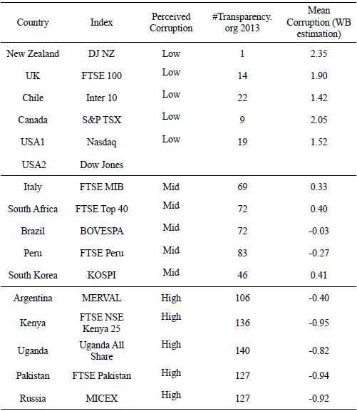
Source: Author's own elaboration.

The first step is to estimate the breaks of the financial indexes series using a wide variety of tests and specifications. Afterwards we estimate Regime Markov Switching models. In this particular case, given the interest in volatility, the model is specified to switch regimes through the variance. The third step is to analyze the political and economic news that were thought to be contemporary to the breaks suggested by the break tests used. For this purpose, the main international news portals were read. We analyzed the major economic news (GDP reports, unemployment, mergers, etc.) and main political news (elections, quit of ministers, corruption events, etc.). The news found were classified as good, bad or neutral. News were scored with values between -2 and 2, depending on how well or bad that news would be for the economy being analyzed.

The idea is to contrast the times when the high volatility state probability starts outweighing the low volatility state probability (i. e. the chances of being in a state of increased volatility are higher) with the breaks found. If they were contemporary with the news analyzed, then the evaluation of the effect of the news were taken into account with a dummy variable, with zero value when the volatility does not rise and one otherwise.

Summarizing, the steps followed were:

1. Estimate structural breaks.
2. Estimate a switch in variance with MS⁵.
3. Contemporaneity. Compare results between steps 1 and 4.
4. Search news for the dates where contemporaneity took place.
5. Evaluate the news and generate an index called "balance".
6. Contrast the news index to observe if the break involves an increase or decrease on the volatility, and considering the level of perceived corruption in that country.

The main purpose is trying to illustrate whether there are certain cases where more information in a market generates greater volatility. But particularly, the analysis is focused on understanding if this phenomenon is more pronounced when economies have a higher perception of corruption.

The main fact that can be observed is that volatility appears to be higher in countries where perceived corruption is in the middle of the distribution according to the index developed by transparency.org. That is, the number of times indicating the break was soaring volatility is greater than the number of times indicating the opposite. We should also add that the average of the balance index is higher (more positive) for countries with moderate corruption than for countries with low and high corruption (it is slightly higher in the case of high corruption, but mean tests show that they are not statistically different) and clearly positive. In turn, the average of the balance index that is obtained for the remaining two types is close to zero, slightly positive in one case (0.06 for lower corruption) and negative on the other (-0.1).

Table II. Breaks on the indexes

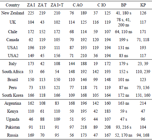
Note 1: ZA denotes the Zivot and Andrews test, C the Clemente et al. test, KP and BP denotes Kim-Perron and Bai-Perron tests respectively. I: intercept, T: trend, AO and IO refers to Additive and Innovative outliers.
Note 2: The numbers displayed refers to the day of the year 2013 when the tests found the break.
Note 3: s: Significant. ns: Not significant.
Source: Author's own elaboration.

Table III. Examples of news labeling

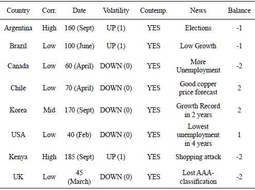
Source: Author's own elaboration.

The results show a Laffer curve for the volatility generated by the news based on the corruption in an economy. This result can be observed on Figure 2.

Countries with middle corruption tend to have higher volatility because of having more positive news (on average).

If two groups of countries are generated, so that on one hand we have moderate corruption countries and on the other hand we have high and low corruption countries together, a simple mean test yields that the difference is significant at 10% (p-value of 0.06). The difference remains significative at 10% even when testing only the average of the moderate group with high or low group average. Finally, the differences are not significative between high and low averages. Potentially more countries in each group can make the results more precise (i.e. rejections on 5 or 1% significance).

Another result is that it appears that in economies with moderate corruption news have a positive mean balance, compared to the average of the full sample. Moreover, we find that good news tend to take place at times with low volatility (average balance of 0.02 versus 0.29 at times of high and low volatility respectively). On the other hand, the other side coin indicates that the average volatility is 0.44 against 0.59 if the balances are positive or negative respectively.

Table IV. Results

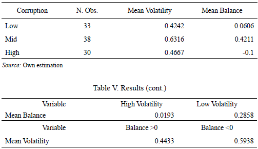
Source: Own estimation

II.3. Extensions and weaknesses of the exercise

Several points can be mentioned about possible modifications and extensions of this approach. First, the sample consisted of an ad hoc selection of 15 countries, and tried to include countries from different continents and cultures in the sample but it is only a sample and therefore the results are conditional to the sample and the period analyzed.

In order to analyze how robust the inverted U shaped curve is more countries from each range could be used (for example 10 countries from each range). However, we should say that in general enough economies were used to represent the overall situation of the world during 2013. We also consider 2013 was a stable year in terms of corruption but our analysis could be extended to any given year or period.

Figure 1. Mean Volatility and Mean Balance

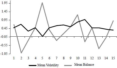
Source: Author's own elaboration.

Figure 2. Mean Volatility and its polynomial mean

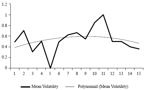
Source: Author's own elaboration.

Second, the findings are also conditional on the balance given to each of the selected news. The impact of this subjectivity is reduced by not using a large range of values. The criterion on the positive or negative news was also conditioned by the editorial focus of the story, but this bias is much lower than the bias generated by the construction of the index.

Finally, a possible extension could be made regarding the methodology. On one hand, different tests of structural breaks were used to make the result more robust but on the other hand we used only MS to estimate regime switches. We might try to include a set of explanatory variables that are the ones that define the threshold. Moreover, we can consider different specifications such as STAR (Auto Regressive Smoothed Transition). The reason for using this narrow switching specification is partly because this is a purely descriptive work and given the absence of a model the choice of explanatory variables would be unjustified.

GENERAL CONCLUSIONS

This paper presents an alternative way to do descriptive analysis. In particular, using econometrics techniques such as break detection and regime estimation and analyzing the possible presence of contemporaneity between economic series.

The general methodological is (i) detect the breaks (ii) estimate the regimes and the switches between them and (iii) analyze contemporaneity between the series breaks and (iv) characterize them with the information obtained from the regimes estimation.

This procedure robustly characterizes the series using several methods, and convergence in results among methodologies is expected.

Our approach presents a new tool attempting to understand the relationship between different time series that may be related but the researcher cannot justify how. We seek to help researchers to explain some sort of causality from a descriptive point of view to find a way to analyze a new connection between variables.

It is worth mentioning that this methodology should be contrasted with standard tools to provide robustness.

Notas
^° Delbianco, F., & Fioriti, A. (2017). Empirical search and characterization of contemporaneity using breaks and regime switching. Estudios económicos, 34 (68), 75-91
¹ See Hamilton (1994) for more details.
² See Pesaran and Timmermann (2000) for example.
³ For the Argentinean case, a 4 years' window should be allowed.
⁴ This is known as T-GARCH, which can isolate asymmetries when to test leverage.
⁵ In this work, the code for MS estimation is from Perlin (2011). These results can be provided upon request.

REFERENCES
1. Acharya, V. V., DeMarzo, P., & Kremer, I. (2011). Endogenous information flows and the clustering of announcements. The American Economic Review, 101 (7), 2955-2979.
2. Bai, J., & Perron, P. (1998). Estimating and Testing Linear Models with Multiple Structural Changes. Econometrica, 66, 47-78.
3. Bai, J. (1997). Estimating multiple breaks one at a time. Econometric Theory, 13 (3), 315-352.
4. Bai, J., & Perron, P. (2003a). Critical values for multiple structural change tests. Econometrics Journal, 6, 7278.
5. Bai, J., & Perron, P. (2003b). Computation and Analysis of Multiple Structural Change Models. Journal of Applied Econometrics, 18, 1-22.
6. Bai, J. & Perron, P. (2006). Multiple Structural Change Models: A Simulation Analysis. In D. Corbae, S. Durlauf, & B. E. Hansen. Econometric Theory and Practice: Frontier of Analysis and Applied Research. Cambridge University Press.
7. Banerjee, A., & Urga, G. (2005). Modelling structural breaks, long memory and stock market volatility: an overview. Journal of Econometrics, 129 (1-2), 1-34.
8. Busetti, F., & Harvey, A. (2001). Testing for the presence of a random walk in series with structural breaks. Journal of Time Series Analysis, 22, 127150.
9. Busetti, F., & Harvey, A. (2003). Further comments on stationarity tests in series with structural breaks. Journal of Time Series Analysis, 24, 137140.
10. Chow, G. C. (1960). Tests of Equality between Sets of Coefficients in Two Linear Regressions. Econometrica, 28 (3), 591-605.
11. Clemente, J., Montañes, A., & Reyes, M. (1998). Testing for a unit root in variables with a double change in the mean. Economics Letters, 59, 175-182.
12. Delbianco, F., & Fioriti, A. (2012). Volatility of the capital flows and structural breaks in Latin America and the Caribbean. Económica, 58, 23-51.
13. Delbianco, F., & Fioriti, A. (2015). Were financial flows in Latin America and the Caribbean shifted by their crises? International Journal of Finance & Economics, 20, 114-125.
14. de Peretti, C., & Urga, G. (2004). Stopping tests in the sequential estimation for multiple structural breaks. Working Paper CEA-06-2004, Centre for Econometric Analysis, Cass Business School, London.
15. Dickey, D., & Fuller, W. (1984). Testing for unit roots in seasonal time series. Journal of the American Statistical Associations, 79, 355-367.
16. Dye, R. (1990). Mandatory versus voluntary disclosures: the cases of financial and real externalities. The Accounting Review, 65 (1), 1-24.
17. Dye, R., & Sridhar, S. (1995). Industry-Wide disclosure dynamics. Journal of Accounting Research, 33 (1), 157-174.
18. Engle, R., & Ng, V. (1993). Measuring and testing the impact of News in Volatility. The Journal of Finance, 48 (5), 1749-1778.
19. Gebka, B. (2012). The Dynamic Relation between Returns, Trading Volume, and Volatility: Lessons from Spillovers between Asia and the United States. Bulletin of Economic Research, 64 (1), 65-90.
20. González, G., & Delbianco, F. (2010). Openness and Total Factor Productivity: Test of Temporal Coincidence of the Structural Breaks for Latin America and the Caribbean. Revista de Análisis Económico, 26 (1), 53-81.
21. Granger, C. W. J. (1969). Investigating Causal Relations by Econometric Models and Cross-spectral Methods. Econometrica, 37 (3), 424438.
22. Hamilton, J. D. (1994). Time Series Analysis. Princeton University Press.
23. Hamilton, J. D. (2005). Regime Switching Models. Palgrave Dictionary of Economics. Retrieved from http://dss.ucsd.edu/~jhamilto/palgrav1.pdf
24. Hansen, B. E. (1990). Lagrange Multiplier Tests for Parameter Instability in Non-Linear Models. Paper presented at The Sixth World Congress of the Econometric Society. University of Rochester, EEUU. Retrieved from http://www.ssc.wisc.edu/~bhansen/papers/LMTests.pdf
25. Hansen, B. E. (1992). Testing for parameter instability in linear models. Journal of Policy Modeling, 14 (4), 517-533.
26. Hansen, B. E. (1997). Approximate asymptotic p-values for structural change tests. Journal of Business and Economic Statistics, 15 (1), 60-67.
27. Hansen, B. E. (2000). Testing for structural change in conditional models. Journal of Econometrics, 97 (1), 93-115.
28. Hansen, B. E. (2001). The New Econometrics of Structural Change: Dating Breaks in U.S. Labor Productivity. The Journal of Economic Perspectives 15 (4), 117-128.
29. Harvey, D., Leybourne, S., & Newbold, P. (2001). Innovational outlier unit root tests with an Endogenously determined break in level. Oxford Bulletin of Economics and Statistics, 63, 559-575.
30. Kaufmann, D., Kraay, A., & Mastruzzi, M. (2010). The Worldwide Governance Indicators: A summary of Methodology, Data and Analytical Issues. World Bank Policy Research, Working Paper No. 5430. Retrieved from http://papers.ssrn.com/sol3/papers.cfm?abstract_id=168213
31. Kim, C., & Nelson, C. (1999). State Space Model with Regime Switching: Classical and Gibbs-Sampling Approaches with Applications. Cambridge, Mass: MIT
32. Press Kim, D., & Perron, P. (2009) Unit Root Tests Allowing for a Break in the Trend Function at an Unknown Time under Both the Null and Alternative Hypotheses. Journal of Econometrics, 148 (1), 1-13.
33. Lee, J., & Strazicich, M. (2001). Break point estimation and spurious rejections with endogenous unit root tests. Oxford Bulletin of Economics and Statistics, 63 (5), 535-558.
34. Maheu, J., & McCurdy, T. (2004). News arrival, jump dynamics, and volatility components for individual stock returns. Journal of Finance, 59 (2), 755-793.
35. Martinez, V. & Rosu, I. (2013). High Frequency Traders, News and Volatility. Working paper. HEC Paris Working Paper.
36. Perlin, M. (2011). MS Regress - The MATLAB Package for Markov Regime Switching Models. Working paper. Retrieve from http://www.stat.ncu.edu.tw/teacher/wenteng/2010%20fall%20teaching/final%20project/Han-Ling%20Yang/MS_Regress_FEX/About%20the%20MS_Regress_Package.pdf
37. Perron, P. (2006). Dealing with Structural Breaks. In T. Mills & K. Patterson (Eds). Palgrave Handbook of Econometrics, Vol. 1: Econometric Theory (278-352). United States: Palgrave Macmillan.
38. Perron, P., & Vogelsang, T. (1992). Testing for a Unit Root in a Time Series with a Changing Mean: Corrections and Extensions. Journal of Business & Economic Statistics, 10 (4), 467-470. doi: 10.2307/1391823
39. Pesaran, H., & Timmermann, A. (2000). Model instability and the choice of observations window. Mimeo, UCSD and University of Cambridge.
40. Pesaran, H., & Timmermann, A. (2005). Small sample properties of forecasts from autoregressive models under structural breaks. Journal of Econometrics, 129 (1-2), 183-217.
41. Zivot, E., & Andrews, D. (1992). Further Evidence on the Great Crash, the Oil Price Shock and the Unit-Root Hypothesis. Journal of Business and Economic Statistics, 10 (3), 251-270.

© 2017 por los autores; licencia otorgada a la revista Estudios económicos. Este artículo es de acceso abierto y distribuido bajo los términos y condiciones de una licencia Atribución-No Comercial 3.0 Unported (CC BY-NC 3.0) de Creative Commons. Para ver una copia de esta licencia, visite http://creativecommons.org/licenses/by-nc/3.0/