Sustainability of the brazilian public debt: an analysis using multicointegration^°

Sostenibilidad de la deuda pública brasileña: un análisis usando multicointegración

Eduardo Lima Campos^* - Rubens Penha Cysne^**

^* EPGE Brazilian School of Economics and Finance (FGV EPGE) and National School of Statistical Science (ENCE/IBGE), Brazil. E-mail: eduardolimacampos@yahoo.com.br
^** EPGE Brazilian School of Economics and Finance (FGV EPGE), Brazil. E-mail: Rubens.Cysne@fgv.br

enviado: 01 noviembre 2019
aceptado: 07 abril 2020

Abstract
According to Bohn (1995), conventional econometric analysis of sustainability, based on unit root tests on the government debt-to-GDP series or cointegration analysis between revenues and expenses, are inconclusive to verify the sustainability of the fiscal policy. This paper uses the multicointegration method to investigate the validity of a long-term relationship between the Brazilian government`s accumulated revenues and expenses and its debt, all expressed as a proportion of GDP. Leachman et al. (2005) argue that this technique allows concluding about the sustainability or not of fiscal policy. The present work considers specifications that allow evaluating the reaction of both accumulated revenues and expenses to changes in the debt-to-GDP, using monthly data from December 1997 to June 2018. We conclude that the Brazilian fiscal policy was unsustainable over the study period, due to the excessive government spending and its growing trajectory, mainly at the end of the sample.

Keywords: Public Debt; Debt Sustainability; Multicointegration.

JEL code: H30, H60, E50.

Resumen
Según Bohn (1995), el análisis econométrico convencional de la sostenibilidad, basado en pruebas de raíz unitaria en la serie de deuda del gobierno al PIB o análisis de cointegración entre ingresos y gastos, no es concluyente para verificar la sostenibilidad de la política fiscal. Este documento utiliza el método de multicointegración para investigar la validez de una relación a largo plazo entre los ingresos y gastos acumulados del gobierno brasileño y su deuda, todo expresado como una proporción del PIB. Leachman et al. (2005) sostienen que esta técnica permite concluir sobre la sostenibilidad o no de la política fiscal. El presente trabajo considera especificaciones que permiten evaluar la reacción de los ingresos y gastos acumulados a los cambios en la deuda con respecto al PIB, utilizando datos mensuales desde diciembre de 1997 hasta junio de 2018. Concluimos que la política fiscal brasileña fue insostenible durante el período de estudio, debido al gasto público excesivo y su trayectoria creciente, principalmente al final de la muestra.

Palabras clave: Deuda Pública; Sostenibilidad de la Deuda; Multicointegración.

Código JEL: H30, H60, E50.

INTRODUCTION¹

A fiscal policy is defined as sustainable if the expected present value of the primary surplus is sufficient to offset the current debt level², or, equivalently, if the government's intertemporal budget constraint is satisfied (Blanchard et al., 1990).

Most of the empirical research on debt sustainability considers two methods. The first one is to test the stationarity of the public debt series (see, for example, Hamilton & Flavin [1986], Wilcox [1989] and Davig [2005]). The second method is the cointegration analysis between the government's revenues and expenses series (see, for example, Trehan & Walsh [1988], Hakkio & Rush [1991], Bohn [1991], Quintos [1995] and, for the Brazilian case, Pastore [1994], Rocha [1997], and Issler & Lima [2000]).

Bohn (1995) criticizes these two approaches, demonstrating that neither the non-rejection of the unit root hypothesis for the debt series, nor the absence of cointegration between the revenues and expenses, are enough to conclude that the debt is unsustainable. According to Bohn, a sustainable fiscal policy is compatible with a debt series integrated of any finite order, which makes it impossible to reject sustainability using these tests.

If the conventional methods do not make it possible to conclude that a fiscal policy is unsustainable, would they be enough to prove sustainability? The answer to this question is also negative. According to Leachman et al. (2005), even if revenues and expenses cointegrate, it is possible that there is an increasing primary deficit (for example, if the government only pays the interest on the debt). In this case, the fiscal policy remains out of control (see, for example, Kia [2008], Kia & Gardner [2011] and Kiran [2011]).

Leachman et al. (2005) show that, to investigate debt sustainability, it is necessary to consider not only the long-term relationship between revenues and expenses series, but also between these variables (accumulated) and the debt stock. The method that allows this type of stock-flow analysis is called multicointegration (Granger and Lee, 1989), and it is applied here to analyze the Brazilian debt sustainability.

I. OBJECTIVES AND CONTRIBUTIONS

This paper aims to investigate the sustainability of Brazilian fiscal policy, using monthly data from December 1997 to June 2018. The multicointegration method is applied to investigate: 1) whether and how accumulated revenues and expenses reacted to Brazilian debt stock variations over the sample; and 2) whether accumulated revenues and expenses and the debt stock are properly balanced - characterizing a sustainable policy - or, at least, whether there is a long-term relationship between revenues and expenses, indicating the so-called weak sustainability (Quintos, 1995). Otherwise, it follows that the fiscal policy was unsustainable over the study period.

Tronzano (2014) adopted variants of this methodology for India, and Camarero et al. (2015) for OECD countries. Both works, however, use the variation of expenses, instead of the debt stock. Triches & Bertussi (2017) apply the method to quarterly Brazilian data (with a specification similar to one of those considered in the present work), and conclude that the debt was weakly sustainable between 1997 and 2015.

Unlike the above articles, we consider not only revenues, but also expenses, as dependent variable. This inversion is coherent with bilateral causality indicated by Granger's causality tests. An additional advantage of the method is the possibility of associating the estimated coefficients with the respective strategy for conducting fiscal policy, and to identify, clearly, which of the variables is responsible for the unsustainability.

Besides, we used the Dickey-Pantula test (1987), the right procedure for investigating the existence of two unit roots in a time series, which is the essential step to investigate the multicointegration hypothesis. The conventional unit root tests, when used for more than one unit root, may lead to wrong conclusions.

Finally, the sample used in this work contemplates the most critical period of Brazilian fiscal policy in recent years, which started in 2014 and lasted at least up to the end of the study period considered here.

The conclusions are different from those reached by Triches & Bertussi (2017), possibly due to the differences in the model specifications and the unit root tests adopted, in addition to the expanded sample.

Our results indicate that the Brazilian fiscal policy was unsustainable throughout the study period, and that main causes of this problem were: 1) the excessive government spending without enough revenue counterpart, and 2) the growing trajectory of expenses, which did not react appropriately to the increasing debt, as expected under a sustainable fiscal policy. The latter conclusion is only possible due to estimation of the alternative model specification considered here, with government expenses as dependent variable.

II. DATA

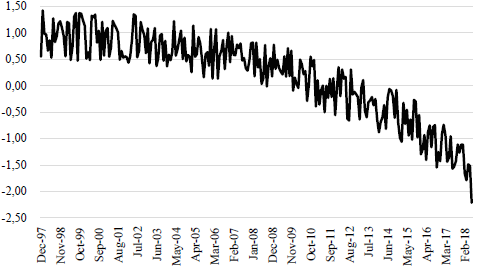
The series used were y_t = revenues³, x_t = total expenses⁴ and net b_t =debt, all for the central government and as a fraction of GDP, from December 1997 to June 2018, obtained on the Brazil Central Bank`s website with monthly frequency. Figure 1 shows the trajectory ofthese variables over the study period (12-months accumulated for easy viewing).

Figure 1. Central Government Revenues, Total Expenses and Net Debt (% of GDP, 12-Months Accumulated, December/1997-June/2018)

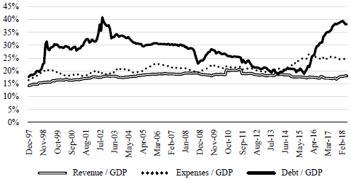
Source: https://www3.bcb.gov.br/sgspub.

It is possible to observe that expenses evolve at a higher level and presents variations of greater amplitude than revenues, over the whole period. A joint evolution of the series is also identified up to the beginning of 2014. From then on, the series detach, with expenses assuming an increasing trajectory throughout 2014 and 2015, and then stabilizing at a higher level until the end of the study period⁵.

The revenues series does not show a noticeable change in its pattern, following a decreasing trajectory in the last years of the sample, slightly growing from the end of 2017 onwards. Finally, the debt series has a stable trajectory up to 2015, when it starts to grow sharply, stabilizing only at the beginning of 2018.

The methodology applied in this work uses accumulated values of y_t and x_t, denoted by: and . Figure 2, below, shows the evolution of these accumulated fiscal variables.

Figure 2. Accumulated Government Revenues and Expenses (% of GDP, December/1997-June/2018)

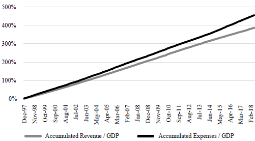
Source: Own elaboration.

It is possible to observe a discrepancy between the trajectories, which is accentuated at the end of the sample, with the accumulated expenses growing faster than the accumulated revenues.

III. METHODOLOGY

III.1. Multicointegration

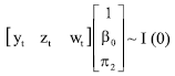
According to Engle & Granger (1987), k series are cointegrated of order (d,b) if: 1) they are integrated in the same order, that is, they are I(d), d > 0; and 2) there is any linear combination of them that is I(d-b), 0 < b ≤ d. Granger & Lee (1989) expand this definition, considering that, for k>2, the series do not need to have the same integration order to have an equilibrium relationship. For example, let's consider three series yt ∼ I(2), z_t ∼ I(2) and w_t ∼ I(1), and suppose we have y_t and z_t cointegrated of order (2,1), that is:

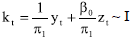(1)

If, in addition, k_t and w_t are cointegrated of order (1,1), that is: 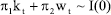, then y_t, z_t, and w_t are said to be multicointegrated. An alternative way of defining multicointegration is to directly represent the equilibrium relationship between all the series involved, that is:

The multicointegration method is important to analyze equilibrium relationship between flow and stock type variables. In this paper, this methodology is used to investigate a long-term relationship between accumulated revenues and expenses over the study period (that is, and ), and the stock of public debt in relation to GDP (b_t), over the same period.

Leachman et al. (2005) verify that, if Y_t, X_t and ΔX_t are multicointegrated, then the fiscal policy is sustainable.

III.2. Model 1

To evaluate the existence of multicointegration, Haldrup (1994) and Engsted at al. (1997) propose the model: , in which t and t² are linear and quadratic trends⁶ terms, respectively, and ε_t represents the error term. However, given the present work objectives', it is convenient to use the debt stock bt instead of ΔXt, and thus the model (called, henceforth, model 1) becomes:

(1)

Equation (1) makes it possible to test the equilibrium relationship between the flow (revenues and expenses) and stock (debt) variables. Additionally, this specification allows investigating whether, and in which proportion, accumulated government revenues react to variations in both public debt and expenses.

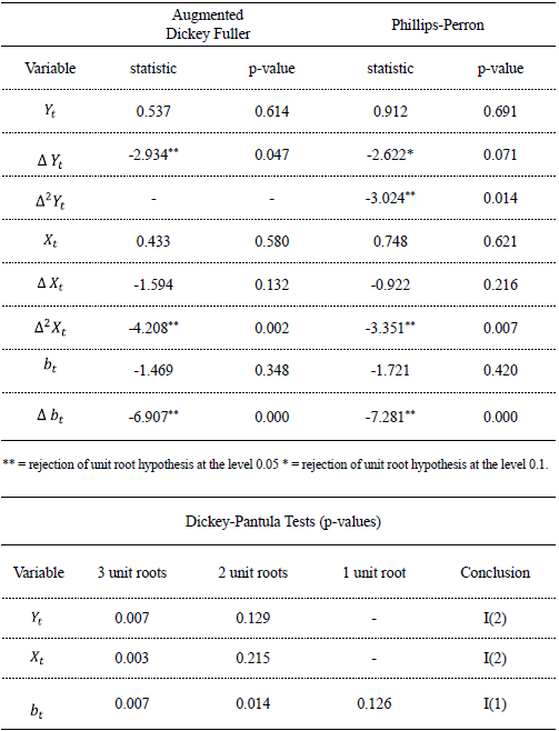
An essential step in this paper is to test the existence of two unit roots, since: 1) it only makes sense to talk of multicointegration if there are at least two I(2) series; and 2) if there is no multicointegration neither cointegration at the first level, the residuals of the estimated model will be I(2). However, according to Dickey & Pantula (1987), the conventional tests, when used to investigate more than one unit root, may lead to find fewer roots than correct⁷. Therefore, the right procedure in this case is to start by testing the existence of d (d > 2) roots; in the case of rejection of this hypothesis, the test is repeated for d-1 roots, and so on. The results of the Dickey-Pantula tests are reported in Annex A, indicating that both Y_t and X_t are I(2), while b_t is I(1), thus confirming the properties required to apply the multicointegration method to these series⁸.

Once equation (1) is estimated, unit root tests must be implemented for the residuals. If they are I(2), it follows that there is no multicointegration, or, equivalently, the fiscal policy is unsustainable. If the residuals are I(1), revenues and expenses are cointegrated in an I(1) order process. In this case, the fiscal policy is classified as weakly sustainable (Quintos, 1995), which means that revenues and expenses evolve together, but they have no long-term relationship with b_t. Thus, they are not reactive to increases in the level of debt. Finally, if is stationary, there is multicointegration, and the Brazilian fiscal policy is said to be sustainable.

A positive aspect of the method is the possibility of direct interpretation of the estimated coefficients, associating them with the strategy for conducting fiscal policy. Specifically, if C₀ > 1, cumulative revenues are higher, on average, than accumulated expenses, leading to the accumulation of surpluses over time; if C₀ = 1, a balanced budget is verified, on average; and if C₀ < 1, expenses tend to accumulate at a higher rate than revenues, which could be a warning for the eminence of debt insolvency. In this last case, fiscal sustainability requires C₁ > 0, in order to ensure that revenues rise as a reaction to the debt increases.

III.3. Model 2

An alternative specification explored in this work is the inversion of revenues and expenses in equation (1), so that X_t becomes the dependent variable. The resulting equation (called, henceforth, model 2) is:

(2)

Equation (2) allows investigating whether, and in which proportion, accumulated government expenses react to variations in both public debt and revenues. This new specification is justified by the following points.

The first justification is that, in Brazil, one of the major fiscal problems is the difficulty to reduce expenses as a way to control the debt increases. This corresponds to X_t not reacting to b_t and Y_t, as in model 2.

The second justification is that X_t considers not only primary expenses, but also the interest on debt, which depends on the debt level and contributes significantly to the expenses, due to the high and volatile interest rates practiced in Brazil. For example, from 2011 to 2015, the Selic ranged from 7.25% to 14.25%.

The third justification is empirical, and it is based on the results of Granger causality tests for cointegrated series, whose results, reported in Annex B, indicate bidirectional causality relationship between cumulative revenues and expenses, in the presence of the debt stock variable.

The interpretation of the C₀ and C₁ parameters is the same as in model 1, reversing revenues and expenses.

Finally, in order to consider the inclusion or not of deterministic terms (t and t²) in the generating process, we estimate constrained and unconstrained versions of equations (1) and (2), which are presented in Table 1 below.

Table 1. Constrained and Unconstrained Specifications for the Models of Equations (1)-(2)

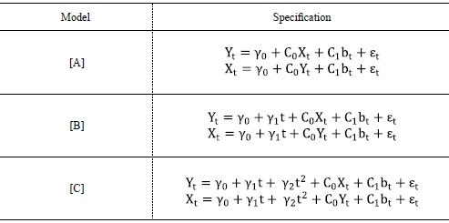
Source: Own elaboration.

IV. RESULTS

IV.1. Model 1 (revenues Y_t as the dependent variable)

Table 2 below presents the results of the multicointegration test (Dickey-Pantula test applied to the residuals) under model 1, according to the specifications of Table 1.

Table 2. Model 1 Estimations and Results of the Multicointegration Tests

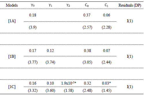
General: . Constrained: and . The values in parentheses represent the t statistic. * = non-significant at the 0.05 level. To formulate the conclusions of the Dickey-Pantula (DP) test, the 0.05 level was considered.
Source: Own elaboration.

The results in Table 2 allow us to conclude that, at the 0.05 level, there is no multicointegration, since the Dickey-Pantula test does not provide evidence in favor of this hypothesis (that is, stationary residuals), under any of the proposed specifications [1A], [1B] or [1C]. On the other hand, the fact that the residuals are I(1) (for all specifications) indicates weak sustainability of fiscal policy, which means that revenues and expenses tend to move together, but there is no long-term relationship between these variables and the debt. Under model 1, it means that revenues did not react (significantly) to changes in the debt stock.

The three specifications presented estimates lower than 1 (around 0.35), indicating that the variations in government expenses exceed, on average, the variations in its revenues, as already identified in Figures 1 and 2. Besides, the positive sign of C₁ suggests that, all else being equal, government revenues reacted to debt increases in the appropriate direction: as the debt grows, an increase in revenues is observed. However, for all specifications, C₁ is lower than 0.1 (not significant in model [1C]), so that the magnitude of the reaction is low and, more importantly, insufficient to put the debt on a sustainable path, in the strong sense⁹.

Specification [1B] has led to the lowest values for the AIC (Akaike information criteria) and BIC (Bayesian information criteria). The residuals of the selected model are presented below:

Figure 3. Model [1B] (Revenues as the dependent variable) Residuals

Source: Own elaboration.

A decreasing trend is clearly observed, reflecting the result of the Dickey-Pantula test, which indicated a first order integrated residuals or the weak sustainability of the Brazilian fiscal policy over the study period.

IV.2. Model 2 (expenses X_t as the dependent variable)

In this section, the results obtained for model 2 are reported, considering expenses as a dependent variable. The coefficient estimates are presented in Table 3 below.

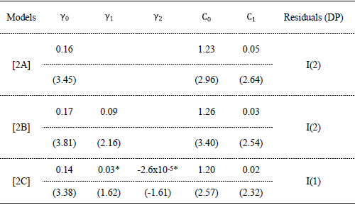
Table 3. Model 2 Estimates and Results of the Multicointegration Tests

General: . Constrained: and . The values in parentheses represent the t statistic. * = non-significant at the 0.05 level. To formulate the conclusions of the Dickey-Pantula (DP) test, the 0.05 level was considered.
Source: Own elaboration.

The three models presented C₀ estimates higher than 1 (around 1.23), confirming the interpretation of this parameter for model 1: the variations in government expenses exceed, on average, the variations in its revenues. Additionally, the positive sign of C₁ suggests that, all else being equal, as the debt grows, an increase (although low) is observed in expenses. This expenses reaction occurs in the opposite direction to that which would be desirable for fiscal controlling. Besides, it is statistically significant at the 0.05 level for all three models.

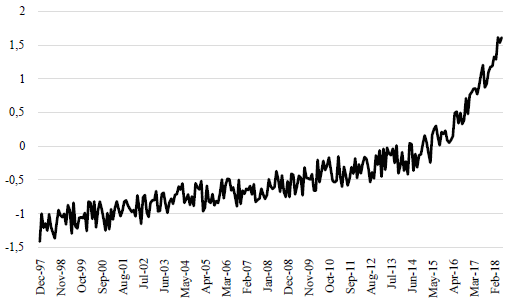
Specification [2B] has led to the lowest values for the AIC and BIC information criteria. As seen, the respective residuals were I(2), indicating that there is no long-term relationship among the variables, even at the first level. The residuals of the selected model are presented below:

Figure 4. Model [2B] (Expenses as the Dependent Variable) Residuals

Source: Own elaboration.

The trend`s accelerated growth and the non-significance of the quadratic deterministic trend in model [2C] are consistent with the second order integrated residuals provided by the Dickey-Pantula test.

It follows that, from the perspective of the reaction of expenses to debt, the Brazilian fiscal policy over the study period cannot be considered sustainable, even in its weak form. It should be emphasized that the alternative use of conventional unit root methods would lead to wrong conclusions, indicating I(1) residuals (see Annex C) and, then, weak sustainability of the fiscal policy. Also here, it is very important to adopt the correct procedure to identify the possibility of more than one unit root, this being one of the present work`s contributions.

CONCLUSIONS

This paper investigated the existence of a long-term relationship between Brazilian central government revenues and expenses accumulated over time and the stock of public debt, all series expressed as a proportion of GDP, applying the multicointegration technique (Granger & Lee, 1989). According to Leachman et al. (2005), this method allows to conclude whether a fiscal policy is sustainable or not, unlike the conventional unit root and cointegration tests usually found in the literature. Both revenues and expenses perspectives were considered.

The results of the multicointegration tests indicate two paths.

From the revenues perspective (model 1), a first level equilibrium relationship is validated, but the multicointegration hypothesis is rejected, that is, there is no stock-flow type relationship between cumulative revenues and expenses and the stock of public debt. Therefore, over the study period, the government did not implement sufficient corrective measures to increase revenues as expenses and the stock of public debt increased. It follows that, from this first perspective, the Brazilian fiscal policy was weakly sustainable throughout the sample.

On the other hand, considering the model for expenses (model 2), we conclude that the fiscal policy did not even present weak sustainability over the study period, which means that the government was unable to control spending as a reaction to debt growth. Besides, the graph of the model 2 residuals indicates that the last years of the sample (2014-2018) seem to have contributed a lot to the unsustainability of fiscal policy.

Finally, the conclusion is that the increase in expenses, without a sufficient revenue counterpart, was responsible for the unsustainability of the public debt in Brazil over the study period. This result agrees perfectly with the current discussion regarding the Brazilian fiscal policy, which emphasizes the need to severely control government spending as the most effective way to put the public debt on a sustainable path.

Annex A. Unit Root Tests for Y_t, X_t and b_t

Source: Own elaboration.

Annex B. Granger Causality Tests for Variables X_t, Y_t and b_t (paired, and always in the presence of the remaining variable)

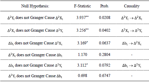
** = causality at the 0.05 level. * = causality at the level 0.1.
Source: Own elaboration.

Annex C. Conventional ADF and Phillips-Perron Unit Root Tests for Model 2 Residuals

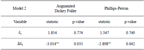
** = rejection of unit root hypothesis at the 0.05 level. * = rejection of unit root at the 0.1 level.
Source: Own elaboration.

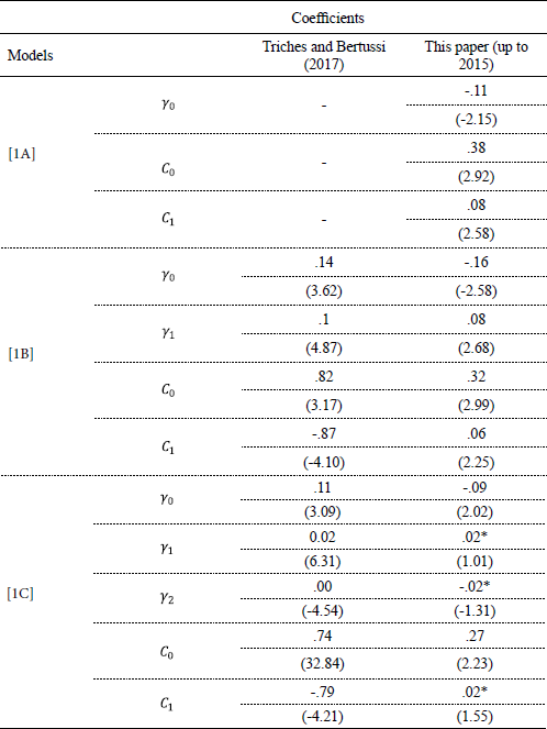
Annex D. Comparison With Triches e Bertussi (2017)

In footnote 9, some divergences were found between our coefficients and those estimated by Triches and Bertussi (2017). For a fair comparison, here the model was implemented for the same time period as the authors, that is, from 1997 to 2015. Thus, the table below presents the results of the multicointegration tests under model 1 estimated for the period from December 1997 to December 2015, in comparison with the results of Triches and Bertussi (2017). It should be highlighted that this author did not implement the [1A] version.

Comparing Our Results With Triches and Bertussi (2017)

The values in parentheses represent the t statistic. * = non-significant at the 0.05 level.
Source: Own elaboration.

Two important differences in relation to Triches and Bertussi (2017) can be highlighted. The first one is the magnitude of the reaction of revenues to the expenses growth, measured by C₀, whose module was lower than 1 in both models (as expected), but presents a substantially smaller magnitude in this paper (0.32x0.82 in model [1B] and 0.27x0.74 in model [1C]). The second difference concerns the reaction of revenues to the public debt growth (C₁ coefficient). While it is negative in the Triches and Bertussi model, it is positive in our model [1B] (although it is not enough to make up for the growth in expenses in the period) and not statistically significant at the 0.05 level in our model [1C]. However, the final conclusion of both models, with common sample, would be the same: weak sustainability. However, it should be noted that Triches and Bertussi (2017) do not consider specification 2, which is essential for one of the main conclusions of the present work.

Notas
^° Campos, E. L., & Cysne, R. P. (2020). Sustainability of the Brazilian public debt: an analysis using multicointegration. Estudios económicos, 37 (75), 5-25.
This study was financed in part by the Coordenação de Aperfeiçoamento de Pessoal de Nível Superior - Brasil (CAPES) - Finance Code 001.
¹ The authors thank Carlos Henrique Dias for his Research Assistance.
² The debt, revenues, expenses, surpluses and deficit series, when not otherwise specified, are always to be considered here as a fraction of GDP.
³ Includes revenues administered or not by the federal government, fiscal incentives and net collections for the General Social Security Regime.
⁴ Personal pensions and charges, executive branch spending, public investments, debt interest and other obligatory spending.
⁵ It is important to highlight that, as of 2015, there was a substantial reduction in interest rates and little variation in GDP. Therefore, the stabilization of the series, in fact, indicates that expenses (not divided by GDP) remained on an increasing trend until the end of the sample.
⁶ The inclusion of deterministic trend is due to the fact that the I(2) variables may present drift in their generating process.
⁷ This mistake - in the case of the test of the residuals of the estimated models - would lead to the wrong conclusion that the fiscal policy is weakly sustainable, whereas in fact it is unsustainable. The problem is that the usual tests consider the existence of at most one unit root.
⁸ Conventional unit root tests (ADF and Philips-Perron), also reported in Annex A, failed to detect the second unit root for the Y_t series.
⁹ Triches & Bertussi (2017), with a similar specification, quarterly data and smaller sample (1997-2015), found and , indicating: 1) lower growth in cumulative expenses in relation to revenues than verified here; and 2) decreasing revenues as the debt increased, an opposite movement to the one verified here. For a fair comparison, Annex D presents the results achieved by estimating our model with the same study period used by the abovementioned authors.

BIBLIOGRAPHY
1. Banco Central do Brasil (2016). Dívida líquida e bruta do governo geral. Retrieved from Sistema Gerenciador de Séries Temporais: https://www3.bcb.gov.br/sgspub
2. Banco Central do Brasil (2016). Relatório de Indicadores Fiscais de junho/2016. Retrieved from https://www.bcb.gov.br/conteudo/home-ptbr/FAQs/FAQ%2004-Indicadores%20Fiscais.pdf
3. Banco Central do Brasil (2016). Sistema Gerenciador de Séries Temporais (código 4189). Retrieved from Sistema Gerenciador de Séries Temporais: https://www3.bcb.gov.br/sgspub
4. Blanchard, O. J., Diamond, P., Hall, R. E., & Murphy, K. (1990). The cyclical behavior of the gross flows of US workers. Brookings Papers on Economic Activity, 1990 (2), 85-155.
5. Bohn, H. (1991). Budget balance through revenue or spending adjustments? Some historical evidence for the United States. Journal of monetary economics, 27 (3), 333-359.
6. Bohn, H. (1995). The Sustainability of Budget Deficits in a Stochastic. Journal of Money, Credit, and Banking, 27 (1), 257-271.
7. Camarero, M., Carrion-i-Silvestre, J., & Tamarit, C. (2015). The relationship between debt level and fiscal sustainability in organization for economic cooperation and development countries. Economic Inquiry, 53 (1), 129-149.
8. Davig, T. (2005). Periodically expanding discounted debt: a threat to fiscal policy sustainability? Journal of Applied Econometrics, 20 (7), 829-840.
9. Dickey, D. A., & Pantula, S. G. (1987). Determining the order of differencing in autoregressive processes. Journal of Business & Economic Statistics, 5 (4), 455-461.
10. Engle, R., & Granger, C. (1987). Co-integration and error correction: representation, estimation, and testing. Econometrica: journal of the Econometric Society, 251-276.
11. Engsted, T., Gonzalo, J. & Haldrup, N. (1997). Testing for Multicointegration. Economics Letters, 56 (3), 259-266.
12. Granger, C. W., & Lee, T. H. (1989). Investigation of production, sales and inventory relationships using multicointegration and non-symmetric error correction models. Journal of applied econometrics, 4 (S1), S145-S159.
13. Hakkio, C. S., & Rush, M. (1991). Is the budget deficit "too large? Economic inquiry, 29 (3), 429-445.
14. Haldrup, N. (1994). The asymptotics of single-equation cointegration regressions with I(1) and I(2) variables. Journal of Econometrics, 63(1), 153-181.
15. Hamilton , J., & Flavin, M. (1986). On the limitations of government borrowing: A framework for empirical testing. American Economic Review, 76 (4), 808-819.
16. IBGE (2016). Retrieved from Séries Históricas e Estatísticas: https://seriesestatisticas.ibge.gov.br/
17. Issler, J. V., & Lima, L. R. (2000). Public debt sustainability and endogenous seigniorage in Brazil: time-series evidence from 1947-1992. Journal of development Economics, 62 (1), 131-147.
18. Johansen, S. (1988). Statistical Analysis of Cointegration Vectors. Journal of Economic Dynamics and Control, 12 (2-3), 231-254.
19. Kia, A. (2008). Fiscal sustainability in emerging countries: Evidence from Iran and Turkey. Journal of Policy Modeling, 30 (6), 957-972.
20. Kia, A., & Gardner, N. (2011). Analysing the fiscal process under a stochastic environment: evidence from Egypt. The Journal of North African Studies, 16 (1), 19-30.
21. Kiran, B. (2011). Sustainability of the fiscal deficit in Turkey: evidence from cointegration and multicointegration tests. International Journal of Sustainable Economy, 3 (1), 63-76.
22. Leachman, L., Bester, A., Rosas, G., & Lange, P. (2005). Multicointegration and Sustainability of Fiscal Practices. Economic Inquiry, 43 (2), 454-466.
23. Pastore, A. C. (1994). Déficit Público, a Sustentabilidade do Crescimento das Dívidas Interna e Externa, Senhoriagem e Inflação: Uma Análise do Regime Monetário Brasileiro. Brazilian Review of Econometrics, 14 (2), 177-234.
24. Quintos, C. E. (1995). Sustainability of the deficit process with structural shifts. Journal of Business & Economic Statistics, 13 (4), 409-417.
25. Rocha, F. (1997). Long-run limits on the Brazilian government debt. Revista brasileira de economia, 51 (4), 447-470.
26. Tesouro Nacional (2016). Various works. Brazil.
27. Trehan, B., & Walsh, C. E. (1988). Common trends, the government's budget constraint, and revenue smoothing. Journal of Economic Dynamics and Control, 12 (2-3), 425-444.
28. Triches, D., & Bertussi, L. S. (2017). Multicointegração e sustentabilidade da política fiscal no Brasil com regime de quebras estruturais (1997-2015). Revista Brasileira de Economia, 71 (3), 379-394.
29. Tronzano, M. (2014). Multicointegration and fiscal sustainability in India: evidence from standard and regime shifts models. Economia internazionale, 67 (2), 263-291.
30. Wilcox, D. W. (1989). The sustainability of government deficits: Implications of the present-value borrowing constraint. Journal of Money, credit and Banking, 21 (3), 291-306.

© 2020 por los autores; licencia no exclusiva otorgada a la revista Estudios económicos. Este artículo es de acceso abierto y distribuido bajo los términos y condiciones de una licencia Atribución-No Comercial 4.0 Internacional (CC BY-NC 4.0) de Creative Commons. Para ver una copia de esta licencia, visite http://creativecommons.org/licenses/by-nc/4.0